Sorting data set 20000421 tetrode D1 (channels 9, 10, 11, 12)
Table of Contents
- 1. Introduction
- 2. Tetrode D1 (channels 9, 10, 11, 12) analysis
- 2.1. Loading the data
- 2.2. Five number summary
- 2.3. Plot the data
- 2.4. Data normalization
- 2.5. Spike detection
- 2.6. Cuts
- 2.7. Events
- 2.8. Removing obvious superposition
- 2.9. Dimension reduction
- 2.10. Exporting for
GGobi - 2.11. kmeans clustering with 6 and 5 clusters
- 2.12. Long cuts creation
- 2.13. Peeling
- 2.14. Getting the spike trains
- 2.15. Getting the inter spike intervals and the forward and backward recurrence times
- 2.16. Testing
all_at_once
- 3. Analyzing a sequence of trials
- 4. Systematic analysis of the 30 trials from
1-Hexanol - 5. 25 trials with
Hexanal - 6. 25 trials with
Cis-3-Hexen-1-ol - 7. 25 trials with
Trans-2-Hexen-1-ol - 8. 25 trials with
1-Hexen-3-ol - 9. 25 trials with
3-Pentanone - 10. 25 trials with
1-Heptanol - 11. 25 trials with
1-Octanol (10^-0) first - 12. 25 trials with
2-Heptanone - 13. 25 trials with
3-Heptanone - 14. 25 trials with
Citral - 15. 25 trials with
Apple - 16. 25 trials with
Mint - 17. 25 trials with
Strawberry - 18. 25 trials with
Amyl Acetate - 19. 25 trials with
Octaldehyde - 20. 25 trials with
1-Octanol (10^-5) - 21. 25 trials with
1-Octanol (10^-4) - 22. 25 trials with
1-Octanol (10^-3) - 23. 25 trials with
1-Octanol (10^-2) - 24. 25 trials with
1-Octanol (10^-1) - 25. 25 trials with
1-Octanol (10^-0) second
1 Introduction
This is the description of how to do the (spike) sorting of tetrode D1 (channels 9, 10, 11, 12) from data set locust20000421.
1.1 Getting the data
The data are in file locust20000421.hdf5 located on zenodo and can be downloaded interactivelly with a web browser or by typing at the command line:
wget https://zenodo.org/record/21589/files/locust20000421.hdf5
In the sequel I will assume that R has been started in the directory where the data were downloaded (in other words, the working direcory should be the one containing the data.
The data are in HDF5 format and the easiest way to get them into R is to install the rhdf5 package from Bioconductor. Once the installation is done, the library is loaded into R with:
library(rhdf5)
We can then get a (long and detailed) listing of our data file content with (result not shown):
h5ls("locust20000421.hdf5")
We can get the content of LabBook metadata from the shell with:
h5dump -a "LabBook" locust20000421.hdf5
1.2 Getting the code
The code can be sourced as follows:
source("https://raw.githubusercontent.com/christophe-pouzat/zenodo-locust-datasets-analysis/master/R_Sorting_Code/sorting_with_r.R")
2 Tetrode D1 (channels 9, 10, 11, 12) analysis
We now want to get our "model", that is a dictionnary of waveforms (one waveform per neuron and per recording site). To that end we are going to use the first 60 s of data contained in the Spontaneous Group (in HDF5 jargon).
2.1 Loading the data
So we start by loading the data from channels 9, 10, 11, 12 into R:
lD = rbind(cbind(h5read("locust20000421.hdf5", "/Spontaneous/ch9"),
                 h5read("locust20000421.hdf5", "/Spontaneous/ch10"),
                 h5read("locust20000421.hdf5", "/Spontaneous/ch11"),
                 h5read("locust20000421.hdf5", "/Spontaneous/ch12")))
dim(lD)
| 892928 |
| 4 |
2.2 Five number summary
We get the Five number summary with:
summary(lD,digits=2)
| Min. : 746 | Min. :1653 | Min. :1497 | Min. :1398 |
| 1st Qu.:2005 | 1st Qu.:1992 | 1st Qu.:2013 | 1st Qu.:2011 |
| Median :2048 | Median :2033 | Median :2055 | Median :2054 |
| Mean :2047 | Mean :2033 | Mean :2054 | Mean :2053 |
| 3rd Qu.:2092 | 3rd Qu.:2074 | 3rd Qu.:2095 | 3rd Qu.:2095 |
| Max. :2996 | Max. :2423 | Max. :2524 | Max. :2581 |
It shows that the channels have very similar properties as far as the median and the inter-quartile range (IQR) are concerned. The minimum is much smaller on the first channel. This suggests that the largest spikes are going to be found here (remember that spikes are going mainly downwards).
2.3 Plot the data
We "convert" the data matrix lD into a time series object with:
lD = ts(lD,start=0,freq=15e3)
We can then plot the whole data with (not shown since it makes a very figure):
plot(lD)
2.4 Data normalization
As always we normalize such that the median absolute deviation (MAD) becomes 1:
lD.mad = apply(lD,2,mad)
lD = t((t(lD)-apply(lD,2,median))/lD.mad)
lD = ts(lD,start=0,freq=15e3)
Once this is done we explore interactively the data with:
explore(lD,col=c("black","grey70"))
Most spikes can be seen on the 4 recording sites and there are different spike waveform!
2.5 Spike detection
Since the spikes are mainly going downwards, we will detect valleys instead of peaks:
lDf = -lD
filter_length = 3
threshold_factor = 4.5
lDf = filter(lDf,rep(1,filter_length)/filter_length)
lDf[is.na(lDf)] = 0
lDf.mad = apply(lDf,2,mad)
lDf_mad_original = lDf.mad
lDf = t(t(lDf)/lDf_mad_original)
thrs = threshold_factor*c(1,1,1,1)
bellow.thrs = t(t(lDf) < thrs)
lDfr = lDf
lDfr[bellow.thrs] = 0
remove(lDf)
sp0 = peaks(apply(lDfr,1,sum),15)
remove(lDfr)
sp0
eventsPos object with indexes of 1184 events.
  Mean inter event interval: 754.31 sampling points, corresponding SD: 861.44 sampling points
  Smallest and largest inter event intervals: 17 and 9283 sampling points.
Every time a filter length / threshold combination is tried, the detection is checked interactively with:
explore(sp0,lD,col=c("black","grey50"))
2.6 Cuts
We proceed as usual to get the cut length right:
evts = mkEvents(sp0,lD,49,50)
evts.med = median(evts)
evts.mad = apply(evts,1,mad)
plot_range = range(c(evts.med,evts.mad))
plot(evts.med,type="n",ylab="Amplitude",
     ylim=plot_range)
abline(v=seq(0,400,10),col="grey")
abline(h=c(0,1),col="grey")
lines(evts.med,lwd=2)
lines(evts.mad,col=2,lwd=2)
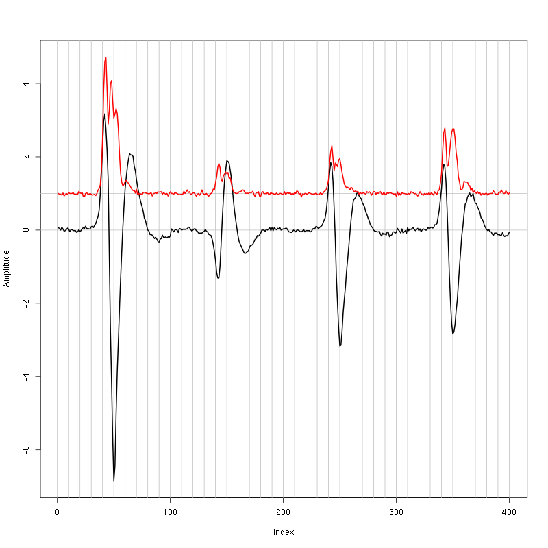
Figure 1: Setting the cut length for the data from tetrode D1 (channels 9, 10, 11, 12). We see that we need 15 points before the peak and 20 after.
We see that we need roughly 15 points before the peak and 20 after.
2.7 Events
We now cut our events:
evts = mkEvents(sp0,lD,14,20)
summary(evts)
events object deriving from data set: lD.
 Events defined as cuts of 35 sampling points on each of the 4 recording sites.
 The 'reference' time of each event is located at point 15 of the cut.
 There are 1184 events in the object.
We can as usual visualize the first 200 events with:
evts[,1:200]
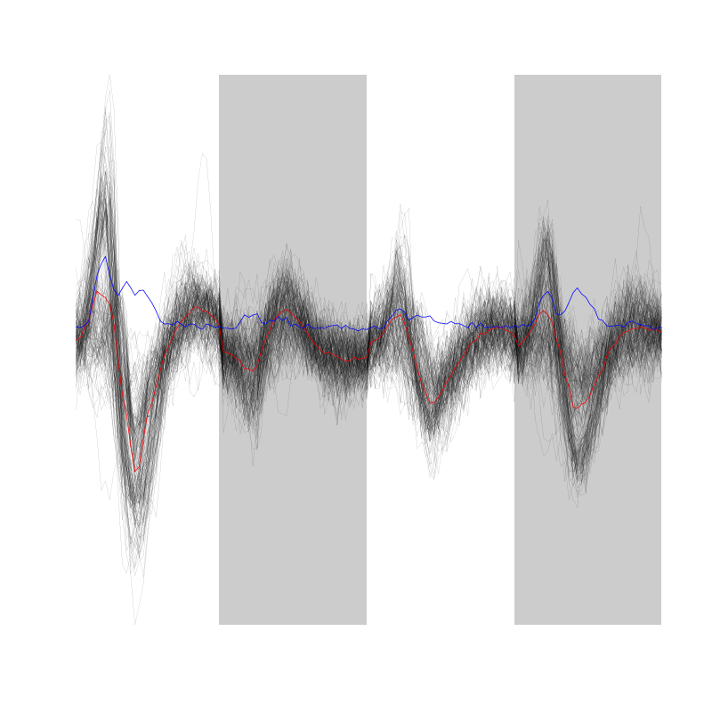
Figure 2: First 200 events for the data from tetrode D1 (channels 1, 3, 5, 7).
There are few superpositions so we try to remove the most obvious ones before doing the dimension reduction.
2.8 Removing obvious superposition
Since some spikes have a pronounced early peak, we will look for superposition only on the late phase (last 10 points) of the events. We define function goodEvtsFct with:
goodEvtsFct = function(samp,thr=3) {
    samp.med = apply(samp,1,median)
    samp.mad = apply(samp,1,mad)
    samp.r = apply(samp,2,function(x) {x[1:25] = 0;x})
    apply(samp.r,2,function(x) all(abs(x-samp.med) < thr*samp.mad))
}
We apply it with a threshold of 4 times the MAD:
goodEvts = goodEvtsFct(evts,4)
2.9 Dimension reduction
We do a PCA on our good events set:
evts.pc = prcomp(t(evts[,goodEvts]))
We look at the projections on the first 4 principle components:
panel.dens = function(x,...) {
  usr = par("usr")
  on.exit(par(usr))
  par(usr = c(usr[1:2], 0, 1.5) )
  d = density(x, adjust=0.5)
  x = d$x
  y = d$y
  y = y/max(y)
  lines(x, y, col="grey50", ...)
}
pairs(evts.pc$x[,1:4],pch=".",gap=0,diag.panel=panel.dens)
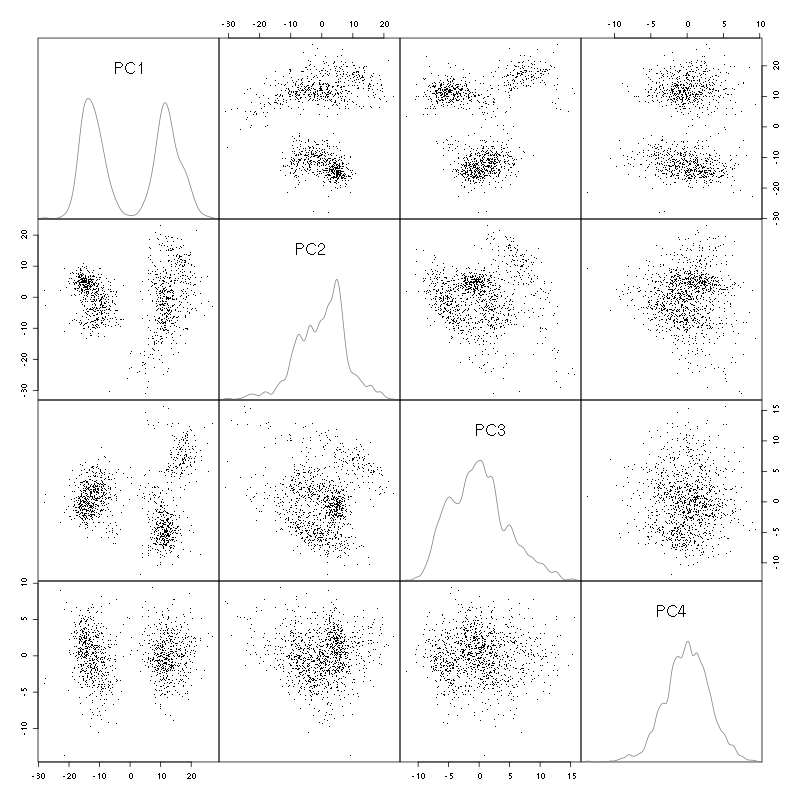
Figure 3: Events from tetrode D1 (channels 9, 10, 11, 12) projected onto the first 4 PCs.
I see at least 4 clusters. We can also look at the projections on the PC pairs defined by the next 4 PCs:
pairs(evts.pc$x[,5:8],pch=".",gap=0,diag.panel=panel.dens)
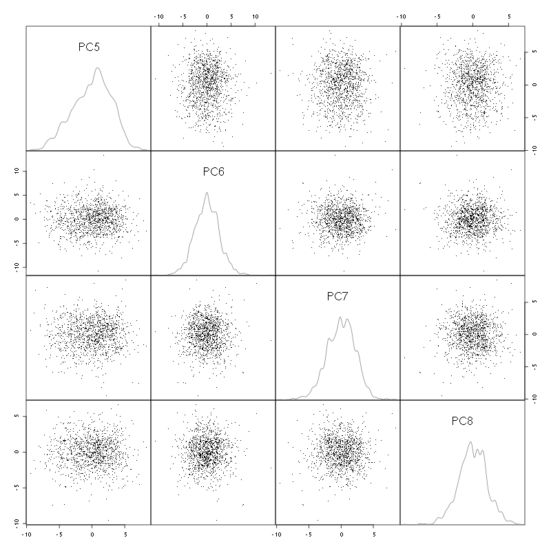
Figure 4: Events from tetrode D1 (channels 9, 10, 11, 12) projected onto PC 5 to 8.
There is not much structure left beyond the 5th PC.
2.10 Exporting for GGobi
We export the events projected onto the first 8 principle components in csv format:
write.csv(evts.pc$x[,1:8],file="tetD1_evts.csv")
Using the rotation display of GGobi with the first 3 principle components and the 2D tour with the first 4 components I see at least 4 clusters but there are probably 5 or 6. So we will start with a kmeans with 5 centers.
2.11 kmeans clustering with 6 and 5 clusters
nbc=6
set.seed(20110928,kind="Mersenne-Twister")
km = kmeans(evts.pc$x[,1:5],centers=nbc,iter.max=100,nstart=100)
label = km$cluster
cluster.med = sapply(1:nbc, function(cIdx) median(evts[,goodEvts][,label==cIdx]))
sizeC = sapply(1:nbc,function(cIdx) sum(abs(cluster.med[,cIdx])))
newOrder = sort.int(sizeC,decreasing=TRUE,index.return=TRUE)$ix
cluster.mad = sapply(1:nbc, function(cIdx) {ce = t(evts[,goodEvts]);ce = ce[label==cIdx,];apply(ce,2,mad)})
cluster.med = cluster.med[,newOrder]
cluster.mad = cluster.mad[,newOrder]
labelb = sapply(1:nbc, function(idx) (1:nbc)[newOrder==idx])[label]
We write a new csv file with the data and the labels:
write.csv(cbind(evts.pc$x[,1:5],labelb),file="tetD1_sorted.csv")
It gives what was expected.
We get a plot showing the events attributed to each unit with:
layout(matrix(1:nbc,nr=nbc))
par(mar=c(1,1,1,1))
for (i in (1:nbc)) plot(evts[,goodEvts][,labelb==i],y.bar=5)
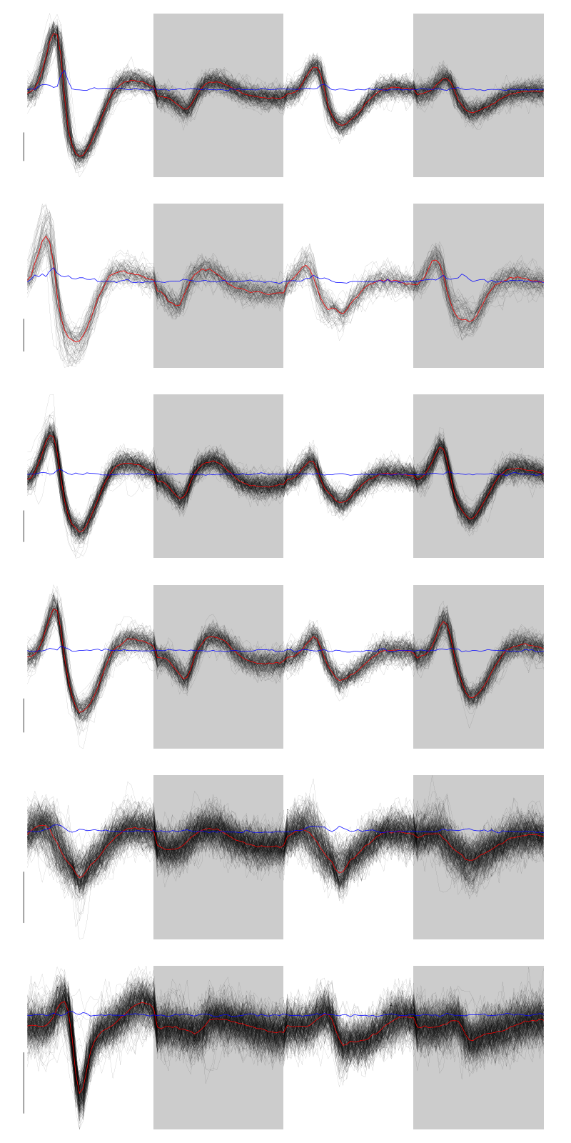
Figure 5: The events of the six clusters of tetrode D1
2, 3 and 4 must be the same. 5 shows evidence that there are at least two neurons, and that some events were missed. We fuse clusters 1 and 2, 3 and 4 and we split 5.
nbc=5
labelb[labelb==3]=2
labelb[labelb==4]=2
kmB = kmeans(evts.pc$x[labelb==5,1:5],centers=2,iter.max=100,nstart=100)
labelB = kmB$cluster
c5_idx = (1:length(labelb))[labelb==5]
for (i in 1:length(c5_idx))
    labelb[c5_idx[i]] = ifelse(labelB[i]==1,3,4)
labelb[labelb==6]=5
We write a new csv file with the data and the labels:
write.csv(cbind(evts.pc$x[,1:5],labelb),file="tetD1b_sorted.csv")
We get a plot showing the events attributed to each unit with:
layout(matrix(1:nbc,nr=nbc))
par(mar=c(1,1,1,1))
for (i in (1:nbc)) {
    ei = labelb==i
    ni = sum(ei)
    plot(evts[,goodEvts][,ei][,1:ifelse(ni>200,200,ni)],y.bar=5)
}
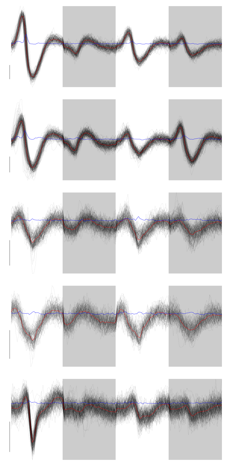
Figure 6: The first 200 events of the five clusters of tetrode D1
2.12 Long cuts creation
For the peeling process we need templates that start and end at 0 (we will otherwise generate artifacts when we subtract). We proceed "as usual" with (I tried first with the default value for parameters before and after but I reduced their values after looking at the centers, see the next figure):
c_before = 49
c_after = 80
centers = lapply(1:nbc, function(i)
    mk_center_list(sp0[goodEvts][labelb==i],lD,
                   before=c_before,after=c_after))
names(centers) = paste("Cluster",1:nbc)
We then make sure that our cuts are long enough by looking at them:
layout(matrix(1:nbc,nr=nbc))
par(mar=c(1,4,1,1))
the_range=c(min(sapply(centers,function(l) min(l$center))),
            max(sapply(centers,function(l) max(l$center))))
for (i in 1:nbc) {
    template = centers[[i]]$center
    plot(template,lwd=2,col=2,
         ylim=the_range,type="l",ylab="")
    abline(h=0,col="grey50")
    abline(v=(1:2)*(c_before+c_after)+1,col="grey50")
    lines(filter(template,rep(1,filter_length)/filter_length),
          col=1,lty=3,lwd=2)
    abline(h=-threshold_factor,col="grey",lty=2,lwd=2)
    lines(centers[[i]]$centerD,lwd=2,col=4)
}
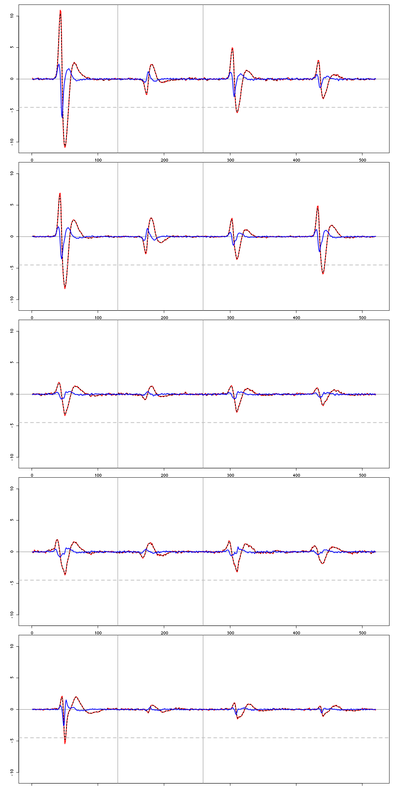
Figure 7: The five templates (red) together with their first derivative (blue) all with the same scale. The dashed black curve show the templates filtered with the filter used during spike detection and the horizontal dashed grey line shows the detection threshold.
Only unit 1 and 2 should reliably pass our threshold, we expect to miss some events from 5, while the other two should be multi-unit…
2.13 Peeling
We can now do the peeling.
2.13.1 Round 0
We classify, predict, subtract and check how many non-classified events we get:
round0 = lapply(as.vector(sp0),classify_and_align_evt,
                data=lD,centers=centers,
                before=c_before,after=c_after)
pred0 = predict_data(round0,centers,data_length = dim(lD)[1])
lD_1 = lD - pred0
sum(sapply(round0, function(l) l[[1]] == '?'))
9
We can see the difference before / after peeling for the data between 1.1 and 1.2 s:
ii = 1:1500 + 1.1*15000
tt = ii/15000
par(mar=c(1,1,1,1))
plot(tt, lD[ii,1], axes = FALSE,
     type="l",ylim=c(-50,10),
     xlab="",ylab="")
lines(tt, lD_1[ii,1], col='red')
lines(tt, lD[ii,2]-15, col='black')
lines(tt, lD_1[ii,2]-15, col='red')
lines(tt, lD[ii,3]-25, col='black')
lines(tt, lD_1[ii,3]-25, col='red')
lines(tt, lD[ii,4]-40, col='black')
lines(tt, lD_1[ii,4]-40, col='red')
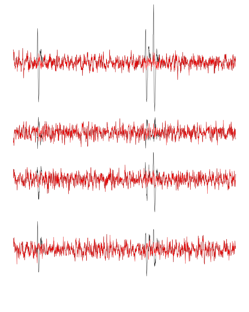
Figure 8: The first peeling illustrated on 100 ms of data, the raw data are in black and the first subtration in red.
2.13.2 Round 1
We keep going, using the subtracted data lD_1 as "raw data", detecting on all sites using the original MAD for normalization and a shorter minimal allowed time between detected spikes:
lDf = -lD_1
lDf = filter(lDf,rep(1,filter_length)/filter_length)
lDf[is.na(lDf)] = 0
lDf = t(t(lDf)/lDf_mad_original)
thrs = threshold_factor*c(1,1,1,1)
bellow.thrs = t(t(lDf) < thrs)
lDfr = lDf
lDfr[bellow.thrs] = 0
remove(lDf)
sp1 = peaks(apply(lDfr,1,sum),10)
remove(lDfr)
sp1
eventsPos object with indexes of 66 events.
  Mean inter event interval: 13465.78 sampling points, corresponding SD: 16215.94 sampling points
  Smallest and largest inter event intervals: 13 and 88036 sampling points.
We classify, predict, subtract and check how many non-classified events we get:
round1 = lapply(as.vector(sp1),classify_and_align_evt,
                data=lD_1,centers=centers,
                before=c_before,after=c_after)
pred1 = predict_data(round1,centers,data_length = dim(lD)[1])
lD_2 = lD_1 - pred1
sum(sapply(round1, function(l) l[[1]] == '?'))
13
We look at what's left with (not shown):
explore(sp1,lD_2,col=c("black","grey50"))
We decide to stop here.
2.14 Getting the spike trains
round_all = c(round0,round1)
spike_trains = lapply(paste("Cluster",1:nbc),
                      function(cn) sort(sapply(round_all[sapply(round_all,
                                                           function(l) l[[1]]==cn)],
                                          function(l) l[[2]]+l[[3]])))
names(spike_trains) = paste("Cluster",1:nbc)
2.15 Getting the inter spike intervals and the forward and backward recurrence times
2.15.1 ISI distributions
We first get the ISI (inter spike intervals) of each unit:
isi = sapply(spike_trains, diff)
names(isi) = names(spike_trains)
We get the ISI ECDF for the five units with:
layout(matrix(1:(nbc+nbc %% 2),nr=ceiling(nbc/2)))
par(mar=c(4,5,6,1))
for (cn in names(isi)) plot_isi(isi[[cn]],main=cn)
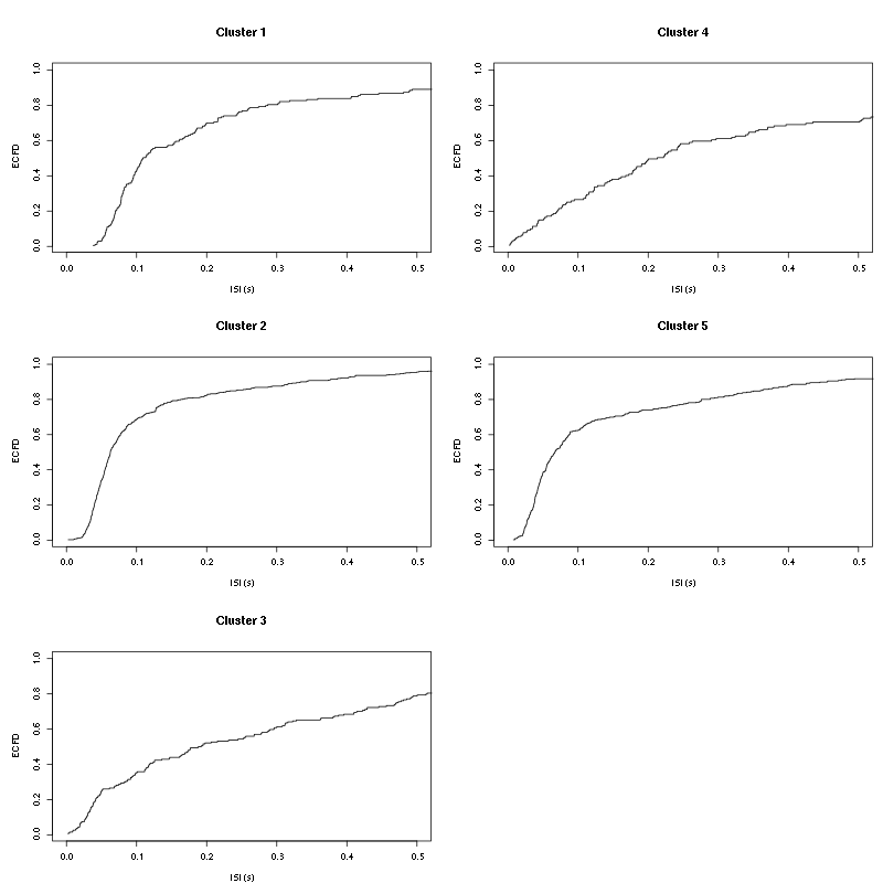
Figure 9: ISI ECDF for the five units.
2.15.2 Forward and Backward Recurrence Times
The forward recurrence time (FRT) between neuron A and B is the elapsed time between a spike in A and the next spike in B. The backward recurrence time (BRT) is the same thing except that we look for the former spike in B. If A and B are not correlated, the expected density of the FRT is the survival function (1-CDF) of the ISI from B divided by the mean ISI of B (the same holds for the BRT under the null hypothesis after taking the opposite). All that is correct if the data are stationary.
On the data at hand that gives:
layout_matrix = matrix(0,nr=nbc,nc=nbc)
counter = 1
for (i in 1:nbc)
    for (j in 1:nbc)
        if (i != j) {
            layout_matrix[i,j] = counter
            counter = counter +1
        }
layout(layout_matrix)
par(mar=c(4,3,4,1))
for (i in 1:nbc)
    for (j in 1:nbc)
        if (i != j)
            test_rt(spike_trains[[i]],
                    spike_trains[[j]],
                    ylab="",main=paste("Units",i,"and",j))
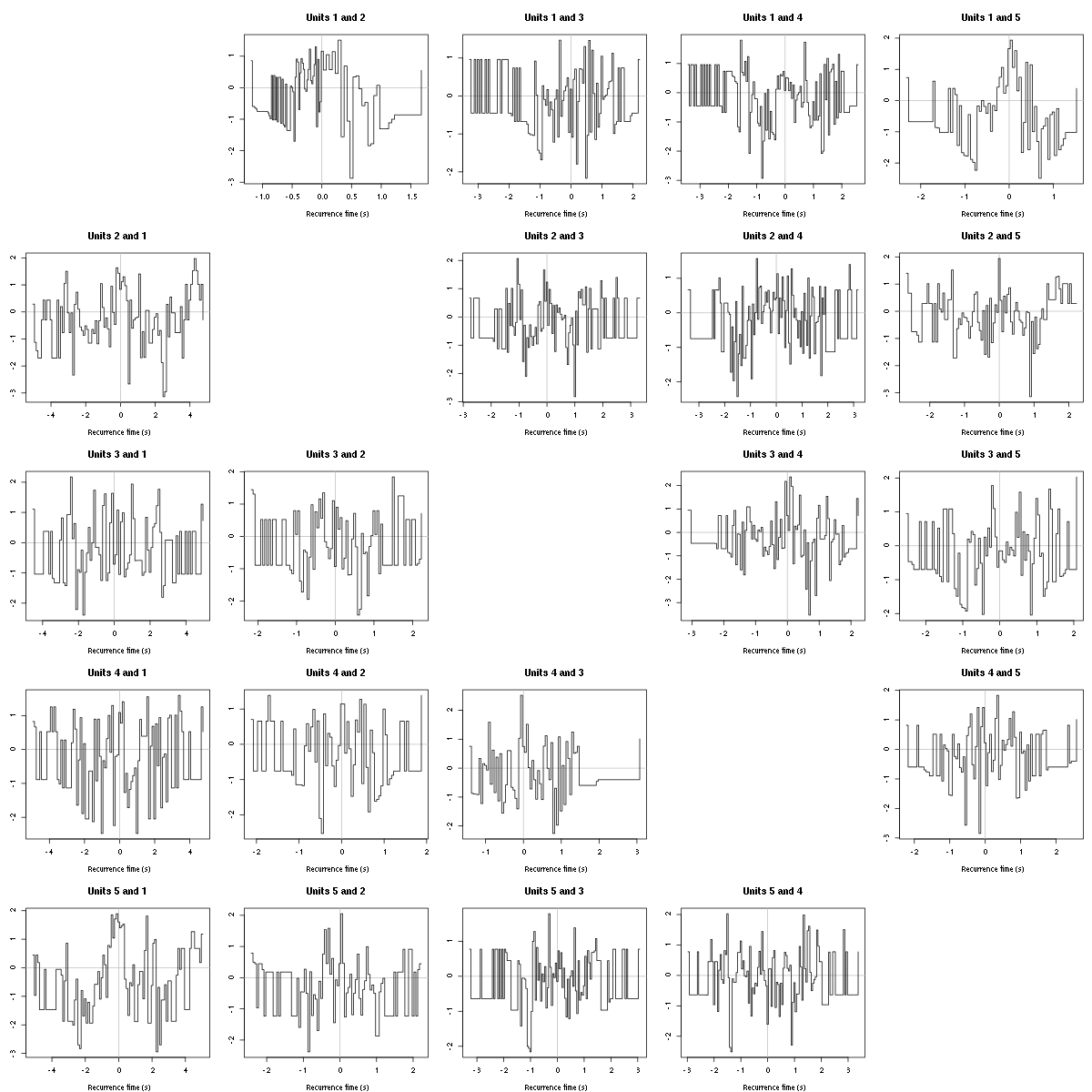
Figure 10: Graphical tests of the Backward and Forward Reccurrence Times distrution agaisnt the null hypothesis (no interaction). If the null is correct, the curves should be IID draws from a standard normal distribution.
2.16 Testing all_at_once
We test the function with:
## We need again an un-normalized version of the data
ref_data = rbind(cbind(h5read("locust20000421.hdf5", "/Spontaneous/ch9"),
                       h5read("locust20000421.hdf5", "/Spontaneous/ch10"),
                       h5read("locust20000421.hdf5", "/Spontaneous/ch11"),
                       h5read("locust20000421.hdf5", "/Spontaneous/ch12")))
## We can now use our function
aao=all_at_once(data=ref_data, centers, thres=threshold_factor*c(1,1,1,1),
                filter_length_1=filter_length, filter_length=filter_length,
                minimalDist_1=15, minimalDist=10,
                before=c_before, after=c_after,
                detection_cycle=c(0,0), verbose=2)
The five number summary is:
       V1             V2             V3             V4
 Min.   : 746   Min.   :1653   Min.   :1497   Min.   :1398
 1st Qu.:2005   1st Qu.:1992   1st Qu.:2013   1st Qu.:2011
 Median :2048   Median :2033   Median :2055   Median :2054
 Mean   :2047   Mean   :2033   Mean   :2054   Mean   :2053
 3rd Qu.:2092   3rd Qu.:2074   3rd Qu.:2095   3rd Qu.:2095
 Max.   :2996   Max.   :2423   Max.   :2524   Max.   :2581

Doing now round 0 detecting on all sites
    Total Cluster 1 Cluster 2 Cluster 3 Cluster 4 Cluster 5         ?
     1184       170       407       174       132       292         9

Doing now round 1 detecting on all sites
    Total Cluster 1 Cluster 2 Cluster 3 Cluster 4 Cluster 5         ?
       66         4         5        11         8        25        13

Global counts at classification's end:
    Total Cluster 1 Cluster 2 Cluster 3 Cluster 4 Cluster 5         ?
     1247       174       412       185       140       317        19
We see that we are getting back the numbers we obtained before step by step.
We can compare the "old" and "new" centers with (not shown):
layout(matrix(1:nbc,nr=nbc))
par(mar=c(1,4,1,1))
for (i in 1:nbc) {
    plot(centers[[i]]$center,lwd=2,col=2,
         ylim=the_range,type="l")
    abline(h=0,col="grey50")
    abline(v=(c_before+c_after)+1,col="grey50")
    lines(aao$centers[[i]]$center,lwd=1,col=4)
}
They are not exactly identical since the new version is computed with all events (superposed or not) attributed to each neuron.
3 Analyzing a sequence of trials
3.1 Create a directory were results get saved
We will carry out an analysis of sequences of 30/25 trials with a given odor. At the end of the analysis of the sequence we will save some intermediate R object in a directory we are now creating.:
if (!dir.exists("tetD1_analysis"))
    dir.create("tetD1_analysis")
3.2 Define a "taylored" version of sort_many_trials
In order to save space and to avoid typos, we define next a taylored version of sort_many_trials:
smt = function(stim_name,
               trial_nbs,
               centers,
               counts) {
    sort_many_trials(inter_trial_time=10*15000,
                     get_data_fct=function(i,s) get_data(i,s,
                                                         channels = c("ch09","ch10","ch11","ch12"),
                                                         file="locust20000421.hdf5"),
                     stim_name=stim_name,
                     trial_nbs=trial_nbs,
                     centers=centers,
                     counts=counts,
                     all_at_once_call_list=list(thres=threshold_factor*c(1,1,1,1),
                                                filter_length_1=filter_length, filter_length=filter_length,
                                                minimalDist_1=15, minimalDist=10,
                                                before=c_before, after=c_after,
                                                detection_cycle=c(0,0), verbose=1),
                     layout_matrix=matrix(1:6,nr=3),new_weight_in_update=0.01
                     )
}
4 Systematic analysis of the 30 trials from 1-Hexanol
The LabBook mentions that a drop of solution was added at trial 13 but looking at the data, no major corruption occurs except for a very sharp artifact so we keep that trial.
4.1 Doing the job
a_1_Hexanol_tetD1=smt(stim_name="1-Hexanol",
                      trial_nbs=1:30,
                      centers=aao$centers,
                      counts=aao$counts)
***************
Doing now trial 1 of 1-Hexanol
The five number summary is:
      ch09           ch10           ch11           ch12
 Min.   :1226   Min.   :1697   Min.   :1662   Min.   :1540
 1st Qu.:2004   1st Qu.:1991   1st Qu.:2012   1st Qu.:2011
 Median :2048   Median :2033   Median :2054   Median :2054
 Mean   :2047   Mean   :2034   Mean   :2053   Mean   :2053
 3rd Qu.:2092   3rd Qu.:2076   3rd Qu.:2094   3rd Qu.:2095
 Max.   :3011   Max.   :2382   Max.   :2566   Max.   :2531

Global counts at classification's end:
    Total Cluster 1 Cluster 2 Cluster 3 Cluster 4 Cluster 5         ?
      101         9        30        21        10        30         1
Trial 1 done!
******************
***************
Doing now trial 2 of 1-Hexanol
The five number summary is:
      ch09           ch10           ch11           ch12
 Min.   :1171   Min.   :1702   Min.   :1557   Min.   :1510
 1st Qu.:2004   1st Qu.:1991   1st Qu.:2012   1st Qu.:2011
 Median :2048   Median :2033   Median :2054   Median :2054
 Mean   :2047   Mean   :2034   Mean   :2053   Mean   :2053
 3rd Qu.:2092   3rd Qu.:2075   3rd Qu.:2095   3rd Qu.:2095
 Max.   :2987   Max.   :2391   Max.   :2485   Max.   :2526

Global counts at classification's end:
    Total Cluster 1 Cluster 2 Cluster 3 Cluster 4 Cluster 5         ?
      125         4        42        24        11        40         4
Trial 2 done!
******************
***************
Doing now trial 3 of 1-Hexanol
The five number summary is:
      ch09           ch10           ch11           ch12
 Min.   : 975   Min.   :1683   Min.   :1546   Min.   :1516
 1st Qu.:2003   1st Qu.:1991   1st Qu.:2012   1st Qu.:2010
 Median :2049   Median :2033   Median :2054   Median :2054
 Mean   :2047   Mean   :2034   Mean   :2053   Mean   :2053
 3rd Qu.:2094   3rd Qu.:2076   3rd Qu.:2096   3rd Qu.:2097
 Max.   :3067   Max.   :2404   Max.   :2535   Max.   :2528

Global counts at classification's end:
    Total Cluster 1 Cluster 2 Cluster 3 Cluster 4 Cluster 5         ?
      262        47       101        15        17        75         7
Trial 3 done!
******************
***************
Doing now trial 4 of 1-Hexanol
The five number summary is:
      ch09           ch10           ch11           ch12
 Min.   :1155   Min.   :1686   Min.   :1624   Min.   :1493
 1st Qu.:2004   1st Qu.:1991   1st Qu.:2012   1st Qu.:2011
 Median :2048   Median :2033   Median :2054   Median :2054
 Mean   :2047   Mean   :2034   Mean   :2053   Mean   :2053
 3rd Qu.:2093   3rd Qu.:2075   3rd Qu.:2095   3rd Qu.:2095
 Max.   :3057   Max.   :2409   Max.   :2554   Max.   :2561

Global counts at classification's end:
    Total Cluster 1 Cluster 2 Cluster 3 Cluster 4 Cluster 5         ?
      175        15        56        26        10        67         1
Trial 4 done!
******************
***************
Doing now trial 5 of 1-Hexanol
The five number summary is:
      ch09           ch10           ch11           ch12
 Min.   :1160   Min.   :1670   Min.   :1610   Min.   :1523
 1st Qu.:2004   1st Qu.:1991   1st Qu.:2012   1st Qu.:2011
 Median :2048   Median :2033   Median :2054   Median :2054
 Mean   :2047   Mean   :2034   Mean   :2053   Mean   :2053
 3rd Qu.:2092   3rd Qu.:2076   3rd Qu.:2095   3rd Qu.:2095
 Max.   :2912   Max.   :2398   Max.   :2478   Max.   :2544

Global counts at classification's end:
    Total Cluster 1 Cluster 2 Cluster 3 Cluster 4 Cluster 5         ?
      135         2        72        21        22        17         1
Trial 5 done!
******************
***************
Doing now trial 6 of 1-Hexanol
The five number summary is:
      ch09           ch10           ch11           ch12
 Min.   :1088   Min.   :1703   Min.   :1558   Min.   :1463
 1st Qu.:2004   1st Qu.:1991   1st Qu.:2012   1st Qu.:2011
 Median :2048   Median :2033   Median :2054   Median :2054
 Mean   :2047   Mean   :2034   Mean   :2053   Mean   :2053
 3rd Qu.:2094   3rd Qu.:2076   3rd Qu.:2096   3rd Qu.:2096
 Max.   :3005   Max.   :2431   Max.   :2517   Max.   :2557

Global counts at classification's end:
    Total Cluster 1 Cluster 2 Cluster 3 Cluster 4 Cluster 5         ?
      201        44        75        14         8        56         4
Trial 6 done!
******************
***************
Doing now trial 7 of 1-Hexanol
The five number summary is:
      ch09           ch10           ch11           ch12
 Min.   :1066   Min.   :1705   Min.   :1608   Min.   :1517
 1st Qu.:2004   1st Qu.:1991   1st Qu.:2012   1st Qu.:2011
 Median :2048   Median :2033   Median :2054   Median :2053
 Mean   :2047   Mean   :2034   Mean   :2053   Mean   :2053
 3rd Qu.:2093   3rd Qu.:2076   3rd Qu.:2095   3rd Qu.:2096
 Max.   :3121   Max.   :2459   Max.   :2571   Max.   :2567

Global counts at classification's end:
    Total Cluster 1 Cluster 2 Cluster 3 Cluster 4 Cluster 5         ?
      163        17        60        26        14        44         2
Trial 7 done!
******************
***************
Doing now trial 8 of 1-Hexanol
The five number summary is:
      ch09           ch10           ch11           ch12
 Min.   :1110   Min.   :1703   Min.   :1586   Min.   :1557
 1st Qu.:2003   1st Qu.:1991   1st Qu.:2012   1st Qu.:2011
 Median :2048   Median :2033   Median :2054   Median :2054
 Mean   :2047   Mean   :2034   Mean   :2053   Mean   :2053
 3rd Qu.:2094   3rd Qu.:2076   3rd Qu.:2095   3rd Qu.:2095
 Max.   :3113   Max.   :2363   Max.   :2526   Max.   :2536

Global counts at classification's end:
    Total Cluster 1 Cluster 2 Cluster 3 Cluster 4 Cluster 5         ?
      211        30        68        28        15        67         3
Trial 8 done!
******************
***************
Doing now trial 9 of 1-Hexanol
The five number summary is:
      ch09           ch10           ch11           ch12
 Min.   :1065   Min.   :1670   Min.   :1573   Min.   :1543
 1st Qu.:2003   1st Qu.:1991   1st Qu.:2012   1st Qu.:2010
 Median :2048   Median :2033   Median :2054   Median :2054
 Mean   :2047   Mean   :2034   Mean   :2053   Mean   :2053
 3rd Qu.:2094   3rd Qu.:2076   3rd Qu.:2096   3rd Qu.:2096
 Max.   :3100   Max.   :2393   Max.   :2500   Max.   :2549

Global counts at classification's end:
    Total Cluster 1 Cluster 2 Cluster 3 Cluster 4 Cluster 5         ?
      217        21        73        24        15        83         1
Trial 9 done!
******************
***************
Doing now trial 10 of 1-Hexanol
The five number summary is:
      ch09           ch10           ch11           ch12
 Min.   :1106   Min.   :1711   Min.   :1595   Min.   :1486
 1st Qu.:2003   1st Qu.:1991   1st Qu.:2012   1st Qu.:2011
 Median :2048   Median :2033   Median :2054   Median :2054
 Mean   :2047   Mean   :2034   Mean   :2053   Mean   :2053
 3rd Qu.:2093   3rd Qu.:2076   3rd Qu.:2095   3rd Qu.:2095
 Max.   :3083   Max.   :2386   Max.   :2530   Max.   :2557

Global counts at classification's end:
    Total Cluster 1 Cluster 2 Cluster 3 Cluster 4 Cluster 5         ?
      118        10        47        16         8        36         1
Trial 10 done!
******************
***************
Doing now trial 11 of 1-Hexanol
The five number summary is:
      ch09           ch10           ch11           ch12
 Min.   :1003   Min.   :1703   Min.   :1567   Min.   :1464
 1st Qu.:2003   1st Qu.:1991   1st Qu.:2012   1st Qu.:2010
 Median :2048   Median :2033   Median :2054   Median :2054
 Mean   :2047   Mean   :2034   Mean   :2053   Mean   :2053
 3rd Qu.:2094   3rd Qu.:2076   3rd Qu.:2095   3rd Qu.:2096
 Max.   :3024   Max.   :2413   Max.   :2575   Max.   :2528

Global counts at classification's end:
    Total Cluster 1 Cluster 2 Cluster 3 Cluster 4 Cluster 5         ?
      220        25       111        16        16        50         2
Trial 11 done!
******************
***************
Doing now trial 12 of 1-Hexanol
The five number summary is:
      ch09           ch10           ch11           ch12
 Min.   :1097   Min.   :1731   Min.   :1555   Min.   :1519
 1st Qu.:2004   1st Qu.:1991   1st Qu.:2012   1st Qu.:2011
 Median :2048   Median :2033   Median :2054   Median :2054
 Mean   :2047   Mean   :2034   Mean   :2053   Mean   :2053
 3rd Qu.:2093   3rd Qu.:2076   3rd Qu.:2095   3rd Qu.:2095
 Max.   :3085   Max.   :2390   Max.   :2533   Max.   :2513

Global counts at classification's end:
    Total Cluster 1 Cluster 2 Cluster 3 Cluster 4 Cluster 5         ?
      119         2        44        20         7        44         2
Trial 12 done!
******************
***************
Doing now trial 13 of 1-Hexanol
The five number summary is:
      ch09           ch10           ch11           ch12
 Min.   : 833   Min.   :   0   Min.   :1346   Min.   :1185
 1st Qu.:2003   1st Qu.:1991   1st Qu.:2012   1st Qu.:2011
 Median :2048   Median :2033   Median :2054   Median :2053
 Mean   :2047   Mean   :2034   Mean   :2053   Mean   :2053
 3rd Qu.:2093   3rd Qu.:2076   3rd Qu.:2094   3rd Qu.:2095
 Max.   :4095   Max.   :2795   Max.   :4095   Max.   :4095

Global counts at classification's end:
    Total Cluster 1 Cluster 2 Cluster 3 Cluster 4 Cluster 5         ?
      145        12        37        19        16        57         4
Trial 13 done!
******************
***************
Doing now trial 14 of 1-Hexanol
The five number summary is:
      ch09           ch10           ch11           ch12
 Min.   : 955   Min.   :1741   Min.   :1556   Min.   :1431
 1st Qu.:2003   1st Qu.:1991   1st Qu.:2012   1st Qu.:2011
 Median :2047   Median :2033   Median :2054   Median :2054
 Mean   :2047   Mean   :2034   Mean   :2053   Mean   :2053
 3rd Qu.:2093   3rd Qu.:2076   3rd Qu.:2095   3rd Qu.:2096
 Max.   :3170   Max.   :2384   Max.   :2517   Max.   :2598

Global counts at classification's end:
    Total Cluster 1 Cluster 2 Cluster 3 Cluster 4 Cluster 5         ?
      144         6        74        22         8        31         3
Trial 14 done!
******************
***************
Doing now trial 15 of 1-Hexanol
The five number summary is:
      ch09           ch10           ch11           ch12
 Min.   : 962   Min.   :1644   Min.   :1531   Min.   :1519
 1st Qu.:2003   1st Qu.:1991   1st Qu.:2011   1st Qu.:2011
 Median :2048   Median :2033   Median :2054   Median :2054
 Mean   :2047   Mean   :2034   Mean   :2053   Mean   :2053
 3rd Qu.:2094   3rd Qu.:2076   3rd Qu.:2095   3rd Qu.:2095
 Max.   :3111   Max.   :2405   Max.   :2529   Max.   :2546

Global counts at classification's end:
    Total Cluster 1 Cluster 2 Cluster 3 Cluster 4 Cluster 5         ?
      201        36        62        20        13        65         5
Trial 15 done!
******************
***************
Doing now trial 16 of 1-Hexanol
The five number summary is:
      ch09           ch10           ch11           ch12
 Min.   : 994   Min.   :1685   Min.   :1565   Min.   :1526
 1st Qu.:2004   1st Qu.:1991   1st Qu.:2012   1st Qu.:2011
 Median :2048   Median :2033   Median :2054   Median :2054
 Mean   :2047   Mean   :2034   Mean   :2053   Mean   :2053
 3rd Qu.:2093   3rd Qu.:2076   3rd Qu.:2095   3rd Qu.:2095
 Max.   :3109   Max.   :2446   Max.   :2508   Max.   :2577

Global counts at classification's end:
    Total Cluster 1 Cluster 2 Cluster 3 Cluster 4 Cluster 5         ?
      154        23        56        16         4        53         2
Trial 16 done!
******************
***************
Doing now trial 17 of 1-Hexanol
The five number summary is:
      ch09           ch10           ch11           ch12
 Min.   : 974   Min.   :1673   Min.   :1579   Min.   :1509
 1st Qu.:2003   1st Qu.:1991   1st Qu.:2012   1st Qu.:2010
 Median :2048   Median :2033   Median :2054   Median :2053
 Mean   :2047   Mean   :2034   Mean   :2053   Mean   :2053
 3rd Qu.:2093   3rd Qu.:2076   3rd Qu.:2095   3rd Qu.:2095
 Max.   :3116   Max.   :2419   Max.   :2579   Max.   :2579

Global counts at classification's end:
    Total Cluster 1 Cluster 2 Cluster 3 Cluster 4 Cluster 5         ?
      146        15        54        10        16        49         2
Trial 17 done!
******************
***************
Doing now trial 18 of 1-Hexanol
The five number summary is:
      ch09           ch10           ch11           ch12
 Min.   :1049   Min.   :1715   Min.   :1478   Min.   :1493
 1st Qu.:2003   1st Qu.:1991   1st Qu.:2012   1st Qu.:2010
 Median :2049   Median :2033   Median :2054   Median :2054
 Mean   :2047   Mean   :2034   Mean   :2053   Mean   :2053
 3rd Qu.:2094   3rd Qu.:2076   3rd Qu.:2095   3rd Qu.:2096
 Max.   :3161   Max.   :2469   Max.   :2579   Max.   :2616

Global counts at classification's end:
    Total Cluster 1 Cluster 2 Cluster 3 Cluster 4 Cluster 5         ?
      202        41        63        10        11        74         3
Trial 18 done!
******************
***************
Doing now trial 19 of 1-Hexanol
The five number summary is:
      ch09           ch10           ch11           ch12
 Min.   : 848   Min.   :1722   Min.   :1557   Min.   :1519
 1st Qu.:2002   1st Qu.:1990   1st Qu.:2010   1st Qu.:2010
 Median :2049   Median :2033   Median :2054   Median :2054
 Mean   :2047   Mean   :2034   Mean   :2053   Mean   :2053
 3rd Qu.:2096   3rd Qu.:2076   3rd Qu.:2096   3rd Qu.:2096
 Max.   :3123   Max.   :2443   Max.   :2526   Max.   :2580

Global counts at classification's end:
    Total Cluster 1 Cluster 2 Cluster 3 Cluster 4 Cluster 5         ?
      320        35       115         8        13       142         7
Trial 19 done!
******************
***************
Doing now trial 20 of 1-Hexanol
The five number summary is:
      ch09           ch10           ch11           ch12
 Min.   :1029   Min.   :1679   Min.   :1533   Min.   :1512
 1st Qu.:2003   1st Qu.:1991   1st Qu.:2012   1st Qu.:2011
 Median :2048   Median :2033   Median :2054   Median :2053
 Mean   :2047   Mean   :2034   Mean   :2053   Mean   :2053
 3rd Qu.:2093   3rd Qu.:2076   3rd Qu.:2095   3rd Qu.:2095
 Max.   :3116   Max.   :2364   Max.   :2491   Max.   :2527

Global counts at classification's end:
    Total Cluster 1 Cluster 2 Cluster 3 Cluster 4 Cluster 5         ?
      158        14        70        12        10        50         2
Trial 20 done!
******************
***************
Doing now trial 21 of 1-Hexanol
The five number summary is:
      ch09           ch10           ch11           ch12
 Min.   : 954   Min.   :1699   Min.   :1645   Min.   :1542
 1st Qu.:2004   1st Qu.:1991   1st Qu.:2012   1st Qu.:2011
 Median :2048   Median :2033   Median :2054   Median :2054
 Mean   :2047   Mean   :2034   Mean   :2053   Mean   :2053
 3rd Qu.:2093   3rd Qu.:2076   3rd Qu.:2095   3rd Qu.:2095
 Max.   :3068   Max.   :2425   Max.   :2573   Max.   :2516

Global counts at classification's end:
    Total Cluster 1 Cluster 2 Cluster 3 Cluster 4 Cluster 5         ?
      125         7        67        11         8        32         0
Trial 21 done!
******************
***************
Doing now trial 22 of 1-Hexanol
The five number summary is:
      ch09           ch10           ch11           ch12
 Min.   :1006   Min.   :1694   Min.   :1533   Min.   :1508
 1st Qu.:2003   1st Qu.:1991   1st Qu.:2012   1st Qu.:2011
 Median :2048   Median :2034   Median :2054   Median :2054
 Mean   :2047   Mean   :2034   Mean   :2053   Mean   :2053
 3rd Qu.:2094   3rd Qu.:2076   3rd Qu.:2095   3rd Qu.:2096
 Max.   :3194   Max.   :2419   Max.   :2562   Max.   :2506

Global counts at classification's end:
    Total Cluster 1 Cluster 2 Cluster 3 Cluster 4 Cluster 5         ?
      204        25        87        14        14        59         5
Trial 22 done!
******************
***************
Doing now trial 23 of 1-Hexanol
The five number summary is:
      ch09           ch10           ch11           ch12
 Min.   : 638   Min.   :1727   Min.   :1525   Min.   :1438
 1st Qu.:2004   1st Qu.:1991   1st Qu.:2012   1st Qu.:2011
 Median :2048   Median :2033   Median :2054   Median :2053
 Mean   :2047   Mean   :2034   Mean   :2053   Mean   :2053
 3rd Qu.:2092   3rd Qu.:2076   3rd Qu.:2095   3rd Qu.:2094
 Max.   :3277   Max.   :2439   Max.   :2602   Max.   :2560

Global counts at classification's end:
    Total Cluster 1 Cluster 2 Cluster 3 Cluster 4 Cluster 5         ?
      139        22        40         9        11        54         3
Trial 23 done!
******************
***************
Doing now trial 24 of 1-Hexanol
The five number summary is:
      ch09           ch10           ch11           ch12
 Min.   :1007   Min.   :1660   Min.   :1564   Min.   :1541
 1st Qu.:2004   1st Qu.:1991   1st Qu.:2012   1st Qu.:2011
 Median :2048   Median :2033   Median :2054   Median :2053
 Mean   :2047   Mean   :2034   Mean   :2053   Mean   :2053
 3rd Qu.:2093   3rd Qu.:2076   3rd Qu.:2094   3rd Qu.:2094
 Max.   :3143   Max.   :2357   Max.   :2555   Max.   :2510

Global counts at classification's end:
    Total Cluster 1 Cluster 2 Cluster 3 Cluster 4 Cluster 5         ?
      160        32        44        16         8        56         4
Trial 24 done!
******************
***************
Doing now trial 25 of 1-Hexanol
The five number summary is:
      ch09           ch10           ch11           ch12
 Min.   : 990   Min.   :1693   Min.   :1568   Min.   :1492
 1st Qu.:2004   1st Qu.:1991   1st Qu.:2012   1st Qu.:2011
 Median :2048   Median :2033   Median :2054   Median :2054
 Mean   :2047   Mean   :2034   Mean   :2053   Mean   :2053
 3rd Qu.:2093   3rd Qu.:2076   3rd Qu.:2095   3rd Qu.:2095
 Max.   :3092   Max.   :2385   Max.   :2521   Max.   :2559

Global counts at classification's end:
    Total Cluster 1 Cluster 2 Cluster 3 Cluster 4 Cluster 5         ?
      188        29        67        17         7        63         5
Trial 25 done!
******************
***************
Doing now trial 26 of 1-Hexanol
The five number summary is:
      ch09           ch10           ch11           ch12
 Min.   : 895   Min.   :1678   Min.   :1528   Min.   :1518
 1st Qu.:2004   1st Qu.:1991   1st Qu.:2012   1st Qu.:2011
 Median :2048   Median :2033   Median :2054   Median :2053
 Mean   :2047   Mean   :2034   Mean   :2053   Mean   :2053
 3rd Qu.:2093   3rd Qu.:2076   3rd Qu.:2095   3rd Qu.:2095
 Max.   :3150   Max.   :2388   Max.   :2542   Max.   :2533

Global counts at classification's end:
    Total Cluster 1 Cluster 2 Cluster 3 Cluster 4 Cluster 5         ?
      198        32        66        13        10        74         3
Trial 26 done!
******************
***************
Doing now trial 27 of 1-Hexanol
The five number summary is:
      ch09           ch10           ch11           ch12
 Min.   : 957   Min.   :1650   Min.   :1543   Min.   :1516
 1st Qu.:2003   1st Qu.:1992   1st Qu.:2012   1st Qu.:2011
 Median :2048   Median :2034   Median :2054   Median :2053
 Mean   :2047   Mean   :2034   Mean   :2053   Mean   :2053
 3rd Qu.:2093   3rd Qu.:2076   3rd Qu.:2095   3rd Qu.:2095
 Max.   :3137   Max.   :2385   Max.   :2530   Max.   :2555

Global counts at classification's end:
    Total Cluster 1 Cluster 2 Cluster 3 Cluster 4 Cluster 5         ?
      195        33        57        13         6        81         5
Trial 27 done!
******************
***************
Doing now trial 28 of 1-Hexanol
The five number summary is:
      ch09           ch10           ch11           ch12
 Min.   : 992   Min.   :1636   Min.   :1517   Min.   :1555
 1st Qu.:2004   1st Qu.:1992   1st Qu.:2012   1st Qu.:2011
 Median :2048   Median :2034   Median :2054   Median :2053
 Mean   :2047   Mean   :2034   Mean   :2053   Mean   :2053
 3rd Qu.:2092   3rd Qu.:2075   3rd Qu.:2094   3rd Qu.:2094
 Max.   :3068   Max.   :2379   Max.   :2541   Max.   :2476

Global counts at classification's end:
    Total Cluster 1 Cluster 2 Cluster 3 Cluster 4 Cluster 5         ?
      164        31        51         6        12        61         3
Trial 28 done!
******************
***************
Doing now trial 29 of 1-Hexanol
The five number summary is:
      ch09           ch10           ch11           ch12
 Min.   :1022   Min.   :1697   Min.   :1599   Min.   :1574
 1st Qu.:2005   1st Qu.:1992   1st Qu.:2012   1st Qu.:2011
 Median :2048   Median :2034   Median :2054   Median :2054
 Mean   :2047   Mean   :2034   Mean   :2053   Mean   :2053
 3rd Qu.:2092   3rd Qu.:2075   3rd Qu.:2094   3rd Qu.:2094
 Max.   :3130   Max.   :2384   Max.   :2550   Max.   :2507

Global counts at classification's end:
    Total Cluster 1 Cluster 2 Cluster 3 Cluster 4 Cluster 5         ?
      124        14        58         6         5        38         3
Trial 29 done!
******************
***************
Doing now trial 30 of 1-Hexanol
The five number summary is:
      ch09           ch10           ch11           ch12
 Min.   :1073   Min.   :1753   Min.   :1628   Min.   :1552
 1st Qu.:2005   1st Qu.:1993   1st Qu.:2013   1st Qu.:2012
 Median :2047   Median :2034   Median :2054   Median :2053
 Mean   :2047   Mean   :2034   Mean   :2053   Mean   :2053
 3rd Qu.:2090   3rd Qu.:2074   3rd Qu.:2093   3rd Qu.:2093
 Max.   :3045   Max.   :2374   Max.   :2489   Max.   :2487

Global counts at classification's end:
    Total Cluster 1 Cluster 2 Cluster 3 Cluster 4 Cluster 5         ?
       99         4        34        16         7        34         4
Trial 30 done!
******************
4.2 Diagnostic plots
The counts evolution is:
counts_evolution(a_1_Hexanol_tetD1)
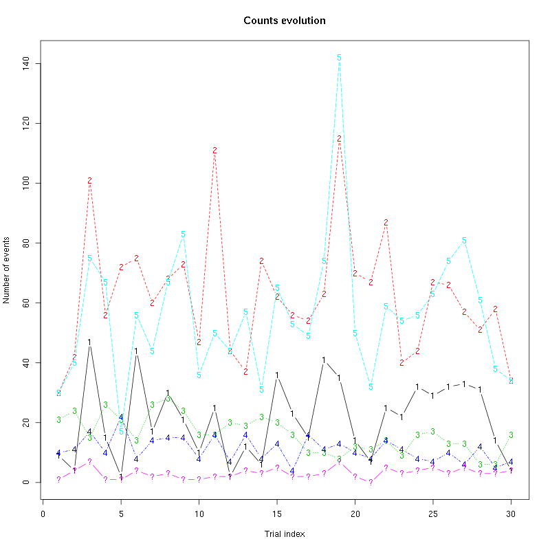
Figure 11: Evolution of the number of events attributed to each unit (1 to 5) or unclassified ("?") during the 30 trials of 1-Hexanol for tetrode D1.
The waveform evolution is:
waveform_evolution(a_1_Hexanol_tetD1,threshold_factor)
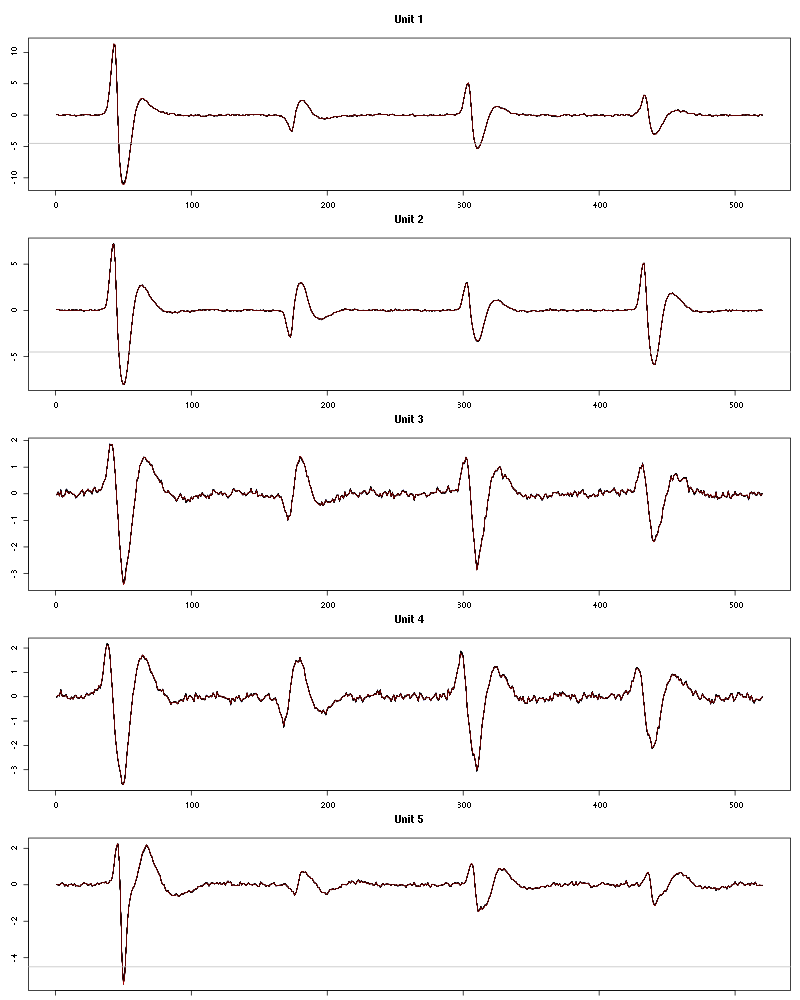
Figure 12: Evolution of the templates of each unit during the 30 trials with 1-Hexanol for tetrode D1.
The observed counting processes, inter spike intervals densities ad raster plots are:
cp_isi_raster(a_1_Hexanol_tetD1)
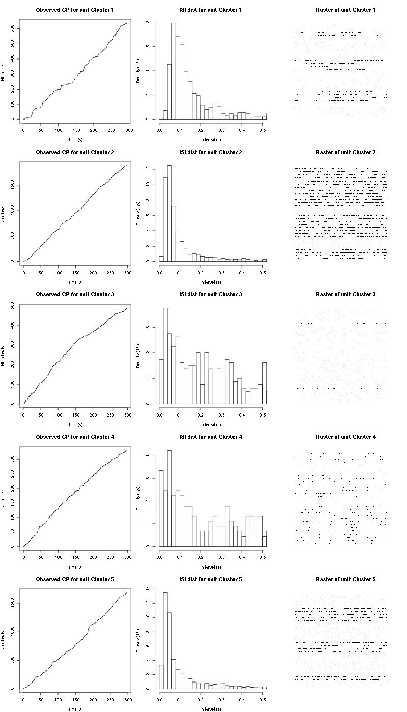
Figure 13: Observed counting processes, empirical inter spike interval distributions and raster plots for 1-Hexanol.
4.3 Save results
Before analyzing the next set of trials we save the output of sort_many_trials to disk with:
save(a_1_Hexanol_tetD1,
     file=paste0("tetD1_analysis/tetD1_","1-Hexanol","_summary_obj.rda"))
We write to disk the spike trains in text mode:
for (c_idx in 1:length(a_1_Hexanol_tetD1$spike_trains))
    cat(a_1_Hexanol_tetD1$spike_trains[[c_idx]],
        file=paste0("locust20000421_spike_trains/locust20000421_1-Hexanol_tetD1_u",c_idx,".txt"),sep="\n")
5 25 trials with Hexanal
We will carry out an analysis of the 25 trials from Hexanal. The LabBook mentions that a drop of solution was added at trial 18 but looking at the data, no major corruption occurs except for a very sharp artifact:
5.1 Do the job
a_Hexanal_tetD1=smt(stim_name="Hexanal",
                    trial_nbs=1:25,
                    centers=a_1_Hexanol_tetD1$centers,
                    counts=a_1_Hexanol_tetD1$counts)
***************
Doing now trial 1 of Hexanal
The five number summary is:
      ch09           ch10           ch11           ch12
 Min.   : 952   Min.   :1720   Min.   :1508   Min.   :1577
 1st Qu.:2005   1st Qu.:1992   1st Qu.:2013   1st Qu.:2011
 Median :2048   Median :2034   Median :2054   Median :2053
 Mean   :2047   Mean   :2034   Mean   :2053   Mean   :2053
 3rd Qu.:2091   3rd Qu.:2075   3rd Qu.:2094   3rd Qu.:2094
 Max.   :3175   Max.   :2409   Max.   :2532   Max.   :2480

Global counts at classification's end:
    Total Cluster 1 Cluster 2 Cluster 3 Cluster 4 Cluster 5         ?
      153        28        26        16        10        65         8
Trial 1 done!
******************
***************
Doing now trial 2 of Hexanal
The five number summary is:
      ch09           ch10           ch11           ch12
 Min.   :1002   Min.   :1676   Min.   :1638   Min.   :1620
 1st Qu.:2005   1st Qu.:1993   1st Qu.:2013   1st Qu.:2012
 Median :2047   Median :2034   Median :2054   Median :2053
 Mean   :2047   Mean   :2034   Mean   :2053   Mean   :2053
 3rd Qu.:2091   3rd Qu.:2075   3rd Qu.:2093   3rd Qu.:2094
 Max.   :3158   Max.   :2356   Max.   :2519   Max.   :2438

Global counts at classification's end:
    Total Cluster 1 Cluster 2 Cluster 3 Cluster 4 Cluster 5         ?
      136        12        23        17        14        66         4
Trial 2 done!
******************
***************
Doing now trial 3 of Hexanal
The five number summary is:
      ch09           ch10           ch11           ch12
 Min.   : 853   Min.   :1733   Min.   :1582   Min.   :1636
 1st Qu.:2005   1st Qu.:1993   1st Qu.:2013   1st Qu.:2012
 Median :2048   Median :2034   Median :2054   Median :2053
 Mean   :2047   Mean   :2034   Mean   :2053   Mean   :2053
 3rd Qu.:2092   3rd Qu.:2075   3rd Qu.:2094   3rd Qu.:2094
 Max.   :3201   Max.   :2329   Max.   :2542   Max.   :2449

Global counts at classification's end:
    Total Cluster 1 Cluster 2 Cluster 3 Cluster 4 Cluster 5         ?
      197        37        18        15         3       116         8
Trial 3 done!
******************
***************
Doing now trial 4 of Hexanal
The five number summary is:
      ch09           ch10           ch11           ch12
 Min.   : 915   Min.   :1765   Min.   :1522   Min.   :1631
 1st Qu.:2004   1st Qu.:1992   1st Qu.:2012   1st Qu.:2012
 Median :2047   Median :2034   Median :2054   Median :2053
 Mean   :2047   Mean   :2034   Mean   :2053   Mean   :2053
 3rd Qu.:2091   3rd Qu.:2075   3rd Qu.:2094   3rd Qu.:2094
 Max.   :3148   Max.   :2419   Max.   :2532   Max.   :2486

Global counts at classification's end:
    Total Cluster 1 Cluster 2 Cluster 3 Cluster 4 Cluster 5         ?
      193        13        18        22         1       137         2
Trial 4 done!
******************
***************
Doing now trial 5 of Hexanal
The five number summary is:
      ch09           ch10           ch11           ch12
 Min.   : 900   Min.   :1766   Min.   :1574   Min.   :1609
 1st Qu.:2004   1st Qu.:1993   1st Qu.:2013   1st Qu.:2011
 Median :2047   Median :2034   Median :2054   Median :2053
 Mean   :2047   Mean   :2034   Mean   :2053   Mean   :2053
 3rd Qu.:2091   3rd Qu.:2075   3rd Qu.:2093   3rd Qu.:2094
 Max.   :3135   Max.   :2353   Max.   :2582   Max.   :2429

Global counts at classification's end:
    Total Cluster 1 Cluster 2 Cluster 3 Cluster 4 Cluster 5         ?
      202        16        30        27         7       114         8
Trial 5 done!
******************
***************
Doing now trial 6 of Hexanal
The five number summary is:
      ch09           ch10           ch11           ch12
 Min.   : 977   Min.   :1721   Min.   :1507   Min.   :1638
 1st Qu.:2005   1st Qu.:1993   1st Qu.:2013   1st Qu.:2012
 Median :2048   Median :2033   Median :2054   Median :2053
 Mean   :2047   Mean   :2034   Mean   :2053   Mean   :2053
 3rd Qu.:2091   3rd Qu.:2075   3rd Qu.:2093   3rd Qu.:2094
 Max.   :3176   Max.   :2364   Max.   :2555   Max.   :2458

Global counts at classification's end:
    Total Cluster 1 Cluster 2 Cluster 3 Cluster 4 Cluster 5         ?
      152        32        34        28         7        41        10
Trial 6 done!
******************
***************
Doing now trial 7 of Hexanal
The five number summary is:
      ch09           ch10           ch11           ch12
 Min.   : 953   Min.   :1651   Min.   :1592   Min.   :1656
 1st Qu.:2005   1st Qu.:1993   1st Qu.:2013   1st Qu.:2012
 Median :2047   Median :2034   Median :2054   Median :2053
 Mean   :2047   Mean   :2034   Mean   :2053   Mean   :2052
 3rd Qu.:2090   3rd Qu.:2074   3rd Qu.:2093   3rd Qu.:2093
 Max.   :3114   Max.   :2364   Max.   :2517   Max.   :2497

Global counts at classification's end:
    Total Cluster 1 Cluster 2 Cluster 3 Cluster 4 Cluster 5         ?
       97        16        13        20         5        42         1
Trial 7 done!
******************
***************
Doing now trial 8 of Hexanal
The five number summary is:
      ch09           ch10           ch11           ch12
 Min.   : 949   Min.   :1715   Min.   :1541   Min.   :1671
 1st Qu.:2005   1st Qu.:1993   1st Qu.:2013   1st Qu.:2012
 Median :2047   Median :2034   Median :2054   Median :2053
 Mean   :2047   Mean   :2034   Mean   :2053   Mean   :2052
 3rd Qu.:2091   3rd Qu.:2074   3rd Qu.:2093   3rd Qu.:2093
 Max.   :3172   Max.   :2391   Max.   :2528   Max.   :2438

Global counts at classification's end:
    Total Cluster 1 Cluster 2 Cluster 3 Cluster 4 Cluster 5         ?
      162        27        20        41         7        58         9
Trial 8 done!
******************
***************
Doing now trial 9 of Hexanal
The five number summary is:
      ch09           ch10           ch11           ch12
 Min.   : 944   Min.   :1733   Min.   :1582   Min.   :1614
 1st Qu.:2005   1st Qu.:1993   1st Qu.:2012   1st Qu.:2012
 Median :2048   Median :2034   Median :2054   Median :2053
 Mean   :2047   Mean   :2034   Mean   :2053   Mean   :2052
 3rd Qu.:2091   3rd Qu.:2075   3rd Qu.:2093   3rd Qu.:2093
 Max.   :3125   Max.   :2410   Max.   :2527   Max.   :2420

Global counts at classification's end:
    Total Cluster 1 Cluster 2 Cluster 3 Cluster 4 Cluster 5         ?
      195        31        22        47        10        79         6
Trial 9 done!
******************
***************
Doing now trial 10 of Hexanal
The five number summary is:
      ch09           ch10           ch11           ch12
 Min.   : 893   Min.   :1737   Min.   :1567   Min.   :1665
 1st Qu.:2005   1st Qu.:1993   1st Qu.:2013   1st Qu.:2012
 Median :2048   Median :2034   Median :2054   Median :2053
 Mean   :2047   Mean   :2034   Mean   :2053   Mean   :2052
 3rd Qu.:2091   3rd Qu.:2075   3rd Qu.:2093   3rd Qu.:2093
 Max.   :3199   Max.   :2353   Max.   :2488   Max.   :2409

Global counts at classification's end:
    Total Cluster 1 Cluster 2 Cluster 3 Cluster 4 Cluster 5         ?
      252        43         8        37        12       146         6
Trial 10 done!
******************
***************
Doing now trial 11 of Hexanal
The five number summary is:
      ch09           ch10           ch11           ch12
 Min.   : 704   Min.   :1722   Min.   :1508   Min.   :1668
 1st Qu.:2005   1st Qu.:1993   1st Qu.:2012   1st Qu.:2012
 Median :2048   Median :2034   Median :2054   Median :2053
 Mean   :2047   Mean   :2034   Mean   :2053   Mean   :2052
 3rd Qu.:2092   3rd Qu.:2074   3rd Qu.:2094   3rd Qu.:2093
 Max.   :3138   Max.   :2383   Max.   :2544   Max.   :2446

Global counts at classification's end:
    Total Cluster 1 Cluster 2 Cluster 3 Cluster 4 Cluster 5         ?
      291        38        12        70        20       139        12
Trial 11 done!
******************
***************
Doing now trial 12 of Hexanal
The five number summary is:
      ch09           ch10           ch11           ch12
 Min.   : 738   Min.   :1641   Min.   :1546   Min.   :1647
 1st Qu.:2006   1st Qu.:1993   1st Qu.:2013   1st Qu.:2012
 Median :2048   Median :2034   Median :2053   Median :2053
 Mean   :2047   Mean   :2034   Mean   :2053   Mean   :2052
 3rd Qu.:2090   3rd Qu.:2074   3rd Qu.:2093   3rd Qu.:2093
 Max.   :3191   Max.   :2377   Max.   :2457   Max.   :2461

Global counts at classification's end:
    Total Cluster 1 Cluster 2 Cluster 3 Cluster 4 Cluster 5         ?
      144        24         7        48        10        51         4
Trial 12 done!
******************
***************
Doing now trial 13 of Hexanal
The five number summary is:
      ch09           ch10           ch11           ch12
 Min.   : 925   Min.   :1743   Min.   :1571   Min.   :1641
 1st Qu.:2006   1st Qu.:1993   1st Qu.:2013   1st Qu.:2012
 Median :2048   Median :2033   Median :2054   Median :2053
 Mean   :2047   Mean   :2034   Mean   :2053   Mean   :2052
 3rd Qu.:2091   3rd Qu.:2074   3rd Qu.:2093   3rd Qu.:2093
 Max.   :3114   Max.   :2348   Max.   :2523   Max.   :2418

Global counts at classification's end:
    Total Cluster 1 Cluster 2 Cluster 3 Cluster 4 Cluster 5         ?
      186        52         5        45         7        69         8
Trial 13 done!
******************
***************
Doing now trial 14 of Hexanal
The five number summary is:
      ch09           ch10           ch11           ch12
 Min.   : 963   Min.   :1751   Min.   :1516   Min.   :1699
 1st Qu.:2005   1st Qu.:1994   1st Qu.:2013   1st Qu.:2012
 Median :2048   Median :2034   Median :2054   Median :2053
 Mean   :2047   Mean   :2034   Mean   :2053   Mean   :2052
 3rd Qu.:2090   3rd Qu.:2074   3rd Qu.:2093   3rd Qu.:2093
 Max.   :3147   Max.   :2366   Max.   :2486   Max.   :2401

Global counts at classification's end:
    Total Cluster 1 Cluster 2 Cluster 3 Cluster 4 Cluster 5         ?
      131        26         5        43         8        46         3
Trial 14 done!
******************
***************
Doing now trial 15 of Hexanal
The five number summary is:
      ch09           ch10           ch11           ch12
 Min.   : 950   Min.   :1661   Min.   :1571   Min.   :1634
 1st Qu.:2006   1st Qu.:1994   1st Qu.:2013   1st Qu.:2012
 Median :2047   Median :2034   Median :2054   Median :2053
 Mean   :2047   Mean   :2034   Mean   :2053   Mean   :2052
 3rd Qu.:2089   3rd Qu.:2074   3rd Qu.:2093   3rd Qu.:2093
 Max.   :3158   Max.   :2339   Max.   :2461   Max.   :2428

Global counts at classification's end:
    Total Cluster 1 Cluster 2 Cluster 3 Cluster 4 Cluster 5         ?
       91         5         5        42         4        31         4
Trial 15 done!
******************
***************
Doing now trial 16 of Hexanal
The five number summary is:
      ch09           ch10           ch11           ch12
 Min.   : 845   Min.   :1726   Min.   :1520   Min.   :1603
 1st Qu.:2006   1st Qu.:1994   1st Qu.:2013   1st Qu.:2012
 Median :2048   Median :2034   Median :2054   Median :2053
 Mean   :2047   Mean   :2034   Mean   :2053   Mean   :2052
 3rd Qu.:2091   3rd Qu.:2074   3rd Qu.:2093   3rd Qu.:2093
 Max.   :3186   Max.   :2348   Max.   :2537   Max.   :2393

Global counts at classification's end:
    Total Cluster 1 Cluster 2 Cluster 3 Cluster 4 Cluster 5         ?
      218        48         2        46        11        99        12
Trial 16 done!
******************
***************
Doing now trial 17 of Hexanal
The five number summary is:
      ch09           ch10           ch11           ch12
 Min.   : 929   Min.   :1726   Min.   :1585   Min.   :1717
 1st Qu.:2006   1st Qu.:1994   1st Qu.:2013   1st Qu.:2012
 Median :2048   Median :2034   Median :2053   Median :2053
 Mean   :2047   Mean   :2034   Mean   :2053   Mean   :2052
 3rd Qu.:2090   3rd Qu.:2074   3rd Qu.:2093   3rd Qu.:2093
 Max.   :3120   Max.   :2343   Max.   :2518   Max.   :2409

Global counts at classification's end:
    Total Cluster 1 Cluster 2 Cluster 3 Cluster 4 Cluster 5         ?
      137        29         2        28        11        64         3
Trial 17 done!
******************
***************
Doing now trial 18 of Hexanal
The five number summary is:
      ch09           ch10           ch11           ch12
 Min.   : 711   Min.   :1084   Min.   :1528   Min.   :1490
 1st Qu.:2005   1st Qu.:1994   1st Qu.:2013   1st Qu.:2012
 Median :2048   Median :2034   Median :2053   Median :2053
 Mean   :2047   Mean   :2034   Mean   :2053   Mean   :2052
 3rd Qu.:2091   3rd Qu.:2074   3rd Qu.:2093   3rd Qu.:2093
 Max.   :3652   Max.   :2586   Max.   :2948   Max.   :2861

Global counts at classification's end:
    Total Cluster 1 Cluster 2 Cluster 3 Cluster 4 Cluster 5         ?
      217        43         1        54        19        88        12
Trial 18 done!
******************
***************
Doing now trial 19 of Hexanal
The five number summary is:
      ch09           ch10           ch11           ch12
 Min.   : 658   Min.   :1717   Min.   :1564   Min.   :1672
 1st Qu.:2006   1st Qu.:1994   1st Qu.:2013   1st Qu.:2012
 Median :2048   Median :2034   Median :2054   Median :2053
 Mean   :2047   Mean   :2034   Mean   :2053   Mean   :2052
 3rd Qu.:2090   3rd Qu.:2074   3rd Qu.:2093   3rd Qu.:2093
 Max.   :3131   Max.   :2331   Max.   :2536   Max.   :2401

Global counts at classification's end:
    Total Cluster 1 Cluster 2 Cluster 3 Cluster 4 Cluster 5         ?
      193        41         3        36        12        88        13
Trial 19 done!
******************
***************
Doing now trial 20 of Hexanal
The five number summary is:
      ch09           ch10           ch11           ch12
 Min.   : 943   Min.   :1743   Min.   :1565   Min.   :1674
 1st Qu.:2006   1st Qu.:1994   1st Qu.:2013   1st Qu.:2012
 Median :2048   Median :2034   Median :2053   Median :2053
 Mean   :2047   Mean   :2034   Mean   :2053   Mean   :2052
 3rd Qu.:2089   3rd Qu.:2074   3rd Qu.:2092   3rd Qu.:2093
 Max.   :3117   Max.   :2413   Max.   :2524   Max.   :2453

Global counts at classification's end:
    Total Cluster 1 Cluster 2 Cluster 3 Cluster 4 Cluster 5         ?
      140        29         0        40        11        54         6
Trial 20 done!
******************
***************
Doing now trial 21 of Hexanal
The five number summary is:
      ch09           ch10           ch11           ch12
 Min.   : 912   Min.   :1718   Min.   :1598   Min.   :1659
 1st Qu.:2006   1st Qu.:1994   1st Qu.:2013   1st Qu.:2012
 Median :2047   Median :2034   Median :2053   Median :2053
 Mean   :2047   Mean   :2034   Mean   :2053   Mean   :2052
 3rd Qu.:2089   3rd Qu.:2074   3rd Qu.:2093   3rd Qu.:2093
 Max.   :3140   Max.   :2364   Max.   :2498   Max.   :2395

Global counts at classification's end:
    Total Cluster 1 Cluster 2 Cluster 3 Cluster 4 Cluster 5         ?
      136        19         4        34         7        59        13
Trial 21 done!
******************
***************
Doing now trial 22 of Hexanal
The five number summary is:
      ch09           ch10           ch11           ch12
 Min.   : 703   Min.   :1717   Min.   :1508   Min.   :1643
 1st Qu.:2006   1st Qu.:1994   1st Qu.:2013   1st Qu.:2012
 Median :2048   Median :2034   Median :2053   Median :2053
 Mean   :2047   Mean   :2034   Mean   :2053   Mean   :2052
 3rd Qu.:2090   3rd Qu.:2074   3rd Qu.:2093   3rd Qu.:2093
 Max.   :3158   Max.   :2358   Max.   :2539   Max.   :2423

Global counts at classification's end:
    Total Cluster 1 Cluster 2 Cluster 3 Cluster 4 Cluster 5         ?
      206        49         1        49        13        87         7
Trial 22 done!
******************
***************
Doing now trial 23 of Hexanal
The five number summary is:
      ch09           ch10           ch11           ch12
 Min.   : 940   Min.   :1759   Min.   :1632   Min.   :1637
 1st Qu.:2006   1st Qu.:1994   1st Qu.:2013   1st Qu.:2012
 Median :2047   Median :2034   Median :2053   Median :2053
 Mean   :2047   Mean   :2034   Mean   :2053   Mean   :2052
 3rd Qu.:2090   3rd Qu.:2074   3rd Qu.:2092   3rd Qu.:2093
 Max.   :3222   Max.   :2376   Max.   :2506   Max.   :2414

Global counts at classification's end:
    Total Cluster 1 Cluster 2 Cluster 3 Cluster 4 Cluster 5         ?
      143        17         0        39         8        77         2
Trial 23 done!
******************
***************
Doing now trial 24 of Hexanal
The five number summary is:
      ch09           ch10           ch11           ch12
 Min.   : 906   Min.   :1740   Min.   :1512   Min.   :1720
 1st Qu.:2006   1st Qu.:1994   1st Qu.:2013   1st Qu.:2012
 Median :2048   Median :2034   Median :2054   Median :2053
 Mean   :2047   Mean   :2034   Mean   :2053   Mean   :2052
 3rd Qu.:2090   3rd Qu.:2074   3rd Qu.:2093   3rd Qu.:2093
 Max.   :3140   Max.   :2405   Max.   :2512   Max.   :2428

Global counts at classification's end:
    Total Cluster 1 Cluster 2 Cluster 3 Cluster 4 Cluster 5         ?
      166        29         2        36         7        85         7
Trial 24 done!
******************
***************
Doing now trial 25 of Hexanal
The five number summary is:
      ch09           ch10           ch11           ch12
 Min.   : 890   Min.   :1695   Min.   :1557   Min.   :1653
 1st Qu.:2005   1st Qu.:1994   1st Qu.:2013   1st Qu.:2012
 Median :2048   Median :2034   Median :2054   Median :2053
 Mean   :2047   Mean   :2034   Mean   :2053   Mean   :2052
 3rd Qu.:2091   3rd Qu.:2074   3rd Qu.:2093   3rd Qu.:2093
 Max.   :3177   Max.   :2402   Max.   :2517   Max.   :2448

Global counts at classification's end:
    Total Cluster 1 Cluster 2 Cluster 3 Cluster 4 Cluster 5         ?
      186        40         1        29        11       101         4
Trial 25 done!
******************
5.2 Diagnostic plots
The counts evolution is:
counts_evolution(a_Hexanal_tetD1)
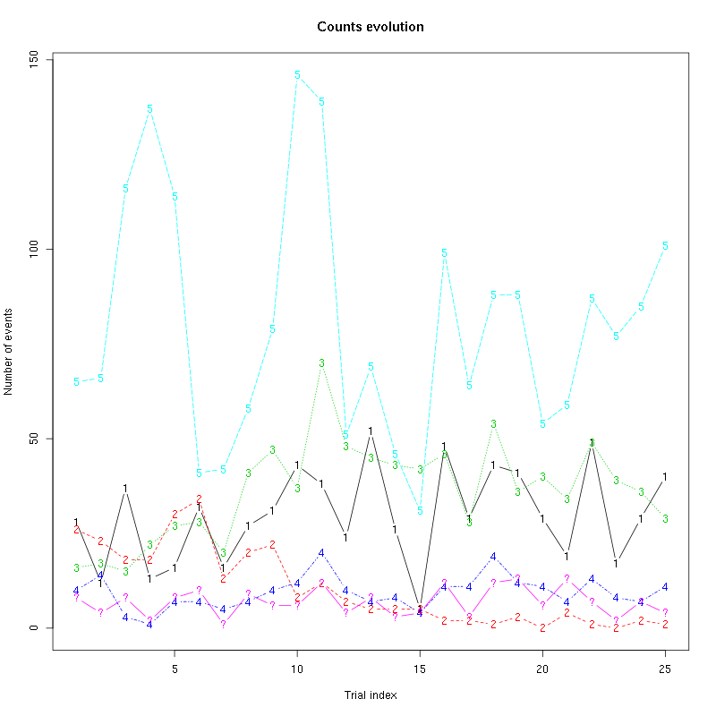
Figure 14: Evolution of the number of events attributed to each unit (1 to 5) or unclassified ("?") during the 25 trials of Hexanal for tetrode D1.
The waveform evolution is:
waveform_evolution(a_Hexanal_tetD1,threshold_factor)
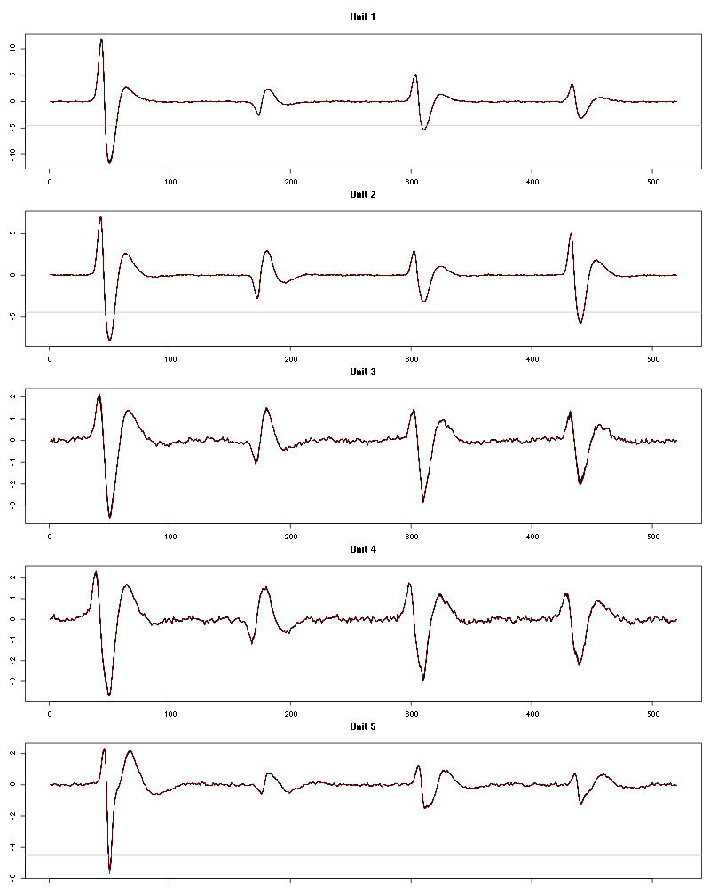
Figure 15: Evolution of the templates of each unit during the 25 trials of Hexanal for tetrode D1.
The observed counting processes, inter spike intervals densities and raster plots are:
cp_isi_raster(a_Hexanal_tetD1)
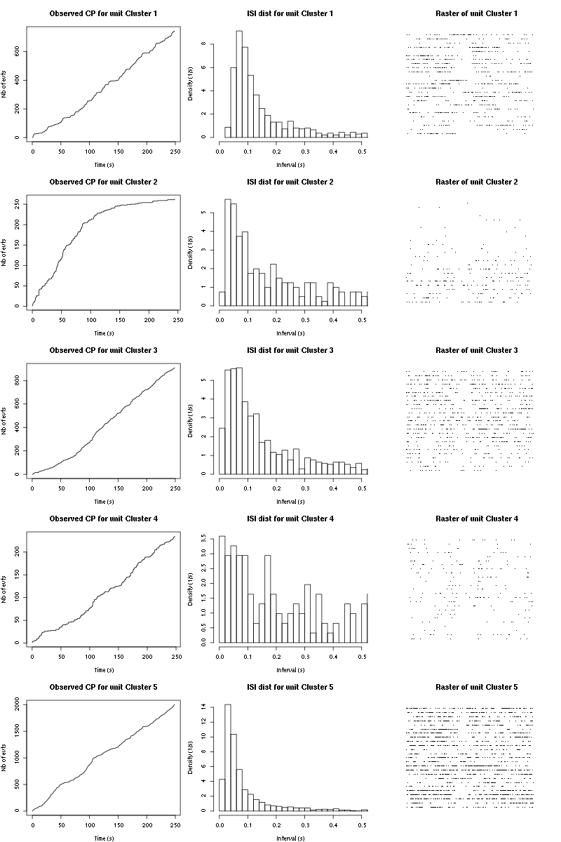
Figure 16: Observed counting processes, empirical inter spike interval distributions and raster plots for Hexanal.
5.3 Save results
Before analyzing the next set of trials we save the output of sort_many_trials to disk with:
save(a_Hexanal_tetD1,
     file=paste0("tetD1_analysis/tetD1_","Hexanal","_summary_obj.rda"))
We write to disk the spike trains in text mode:
for (c_idx in 1:length(a_Hexanal_tetD1$spike_trains))
    cat(a_Hexanal_tetD1$spike_trains[[c_idx]],
        file=paste0("locust20000421_spike_trains/locust20000421_Hexanal_tetD1_u",c_idx,".txt"),sep="\n")
6 25 trials with Cis-3-Hexen-1-ol
We will carry out an analysis of the 25 trials from Cis-3-Hexen-1-ol.
6.1 Do the job
We do not print out the output to save space.
a_Cis_3_Hexen_1_ol_tetD1=smt(stim_name="Cis-3-Hexen-1-ol",
                             trial_nbs=1:25,
                             centers=a_Hexanal_tetD1$centers,
                             counts=a_Hexanal_tetD1$counts)
6.2 Diagnostic plots
The counts evolution is:
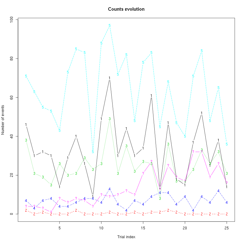
Figure 17: Evolution of the number of events attributed to each unit (1 to 5) or unclassified ("?") during the 30 trials of Cis-3-Hexen-1-ol for tetrode D1.
The waveform evolution is:
waveform_evolution(a_Cis_3_Hexen_1_ol_tetD1,threshold_factor)

Figure 18: Evolution of the templates of each unit during the 25 trials of Cis-3-Hexen-1-ol for stereode Ca.
The observed counting processes, inter spike intervals densities and raster plots are:
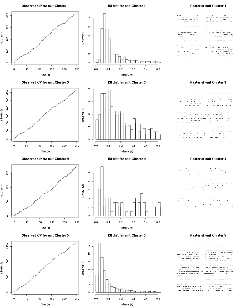
Figure 19: Observed counting processes, empirical inter spike interval distributions and raster plots for Cis-3-Hexen-1-ol.
6.3 Save results
Before analyzing the next set of trials we save the output of sort_many_trials to disk with:
save(a_Cis_3_Hexen_1_ol_tetD1,
     file=paste0("tetD1_analysis/tetD1_","Cis-3-Hexen-1-ol","_summary_obj.rda"))
We write to disk the spike trains in text mode:
for (c_idx in 1:length(a_Cis_3_Hexen_1_ol_tetD1$spike_trains))
    if (!is.null(a_Cis_3_Hexen_1_ol_tetD1$spike_trains[[c_idx]]))
        cat(a_Cis_3_Hexen_1_ol_tetD1$spike_trains[[c_idx]],
	    file=paste0("locust20000421_spike_trains/locust20000421_Cis-3-Hexen-1-ol_tetD1_u",c_idx,".txt"),sep="\n")
7 25 trials with Trans-2-Hexen-1-ol
We will carry out an analysis of the 25 trials from Trans-2-Hexen-1-ol.
7.1 Do the job
stim_name = "Trans-2-Hexen-1-ol"
a_Trans_2_Hexen_1_ol_tetD1=smt(stim_name=stim_name,
                               trial_nbs=1:25,
                               centers=a_Cis_3_Hexen_1_ol_tetD1$centers,
                               counts=a_Cis_3_Hexen_1_ol_tetD1$counts)
7.2 Diagnostic plots
The counts evolution is:
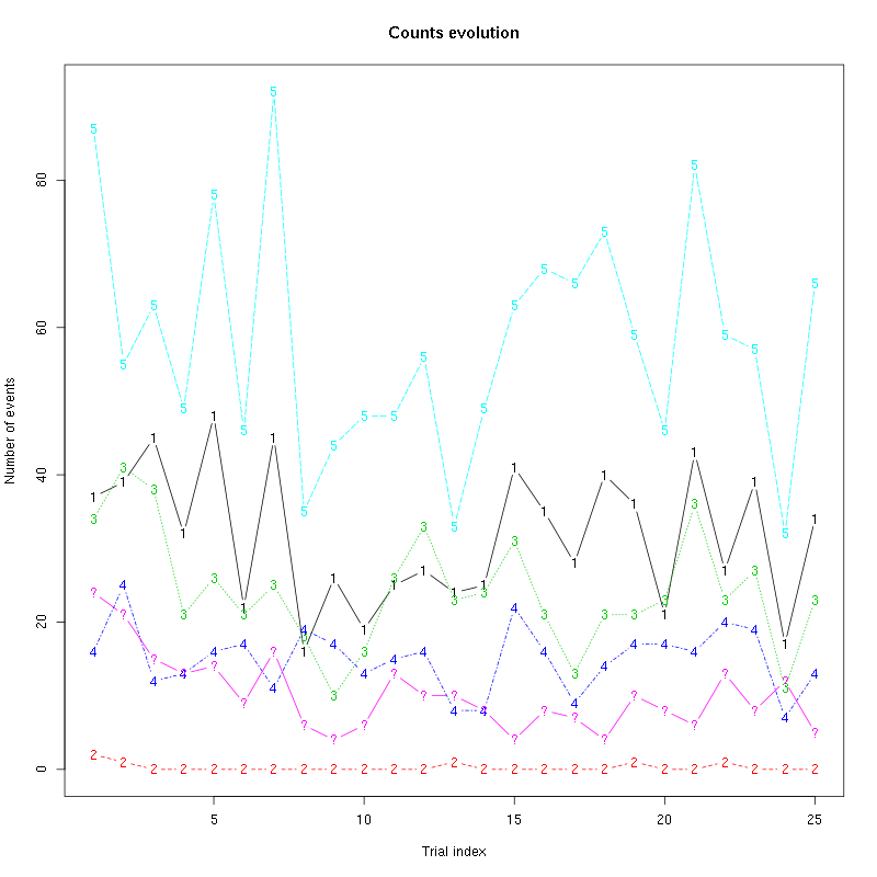
Figure 20: Evolution of the number of events attributed to each unit (1 to 5) or unclassified ("?") during the 25 trials of Trans-2-Hexen-1-ol for tetrodeD1.
The waveform evolution is:
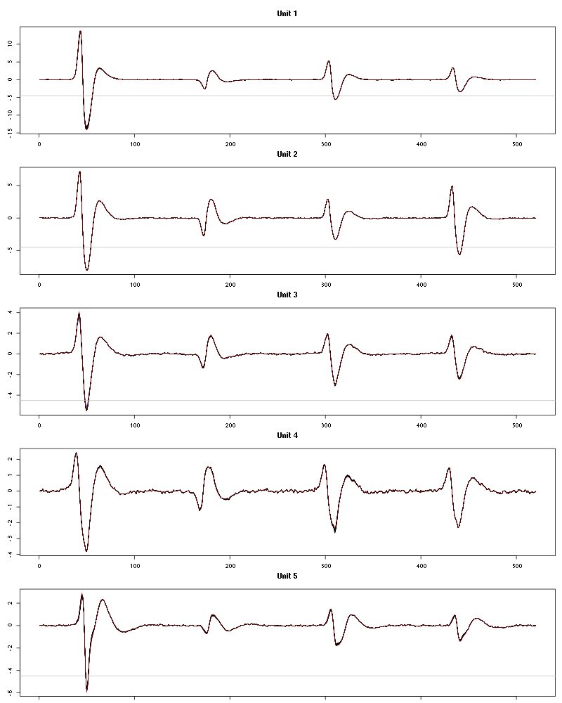
Figure 21: Evolution of the templates of each unit during the 25 trials of Trans-2-Hexen-1-ol for tetrodeD1.
The observed counting processes, inter spike intervals densities and raster plots are:
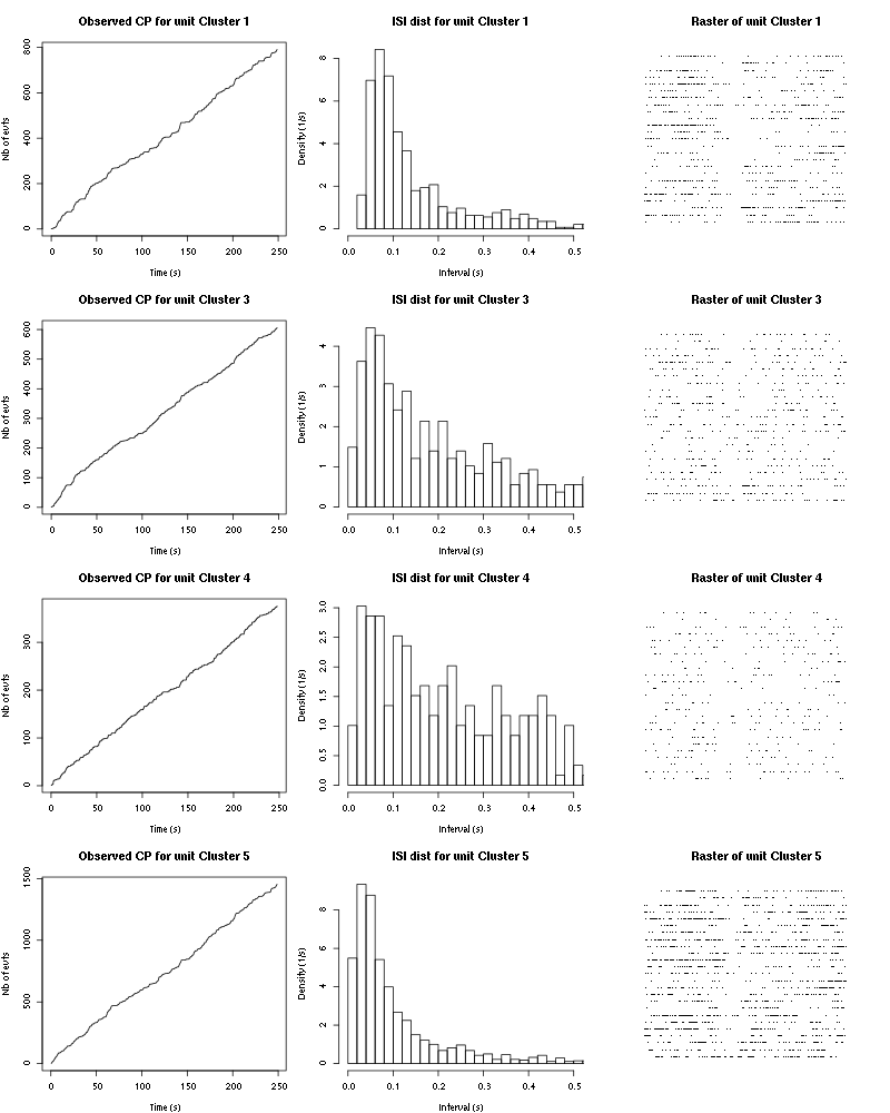
Figure 22: Observed counting processes, empirical inter spike interval distributions and raster plots for Trans-2-Hexen-1-ol.
7.3 Save results
Before analyzing the next set of trials we save the output of sort_many_trials to disk with:
save(a_Trans_2_Hexen_1_ol_tetD1,
     file=paste0("tetD1_analysis/tetD1_",stim_name,"_summary_obj.rda"))
We write to disk the spike trains in text mode:
for (c_idx in 1:length(a_Trans_2_Hexen_1_ol_tetD1$spike_trains))
    if (!is.null(a_Trans_2_Hexen_1_ol_tetD1$spike_trains[[c_idx]]))
        cat(a_Trans_2_Hexen_1_ol_tetD1$spike_trains[[c_idx]],
            file=paste0("locust20000421_spike_trains/locust20000421_Trans-2-Hexen-1-ol_tetD1_u",
                        c_idx,".txt"),sep="\n")
8 25 trials with 1-Hexen-3-ol
We will carry out an analysis of the 25 trials from 1-Hexen-3-ol.
8.1 Do the job
stim_name = "1-Hexen-3-ol"
a_1_Hexen_3_ol_tetD1=smt(stim_name=stim_name,
                         trial_nbs=1:25,
                         centers=a_Trans_2_Hexen_1_ol_tetD1$centers,
                         counts=a_Trans_2_Hexen_1_ol_tetD1$counts)
8.2 Diagnostic plots
The counts evolution is:
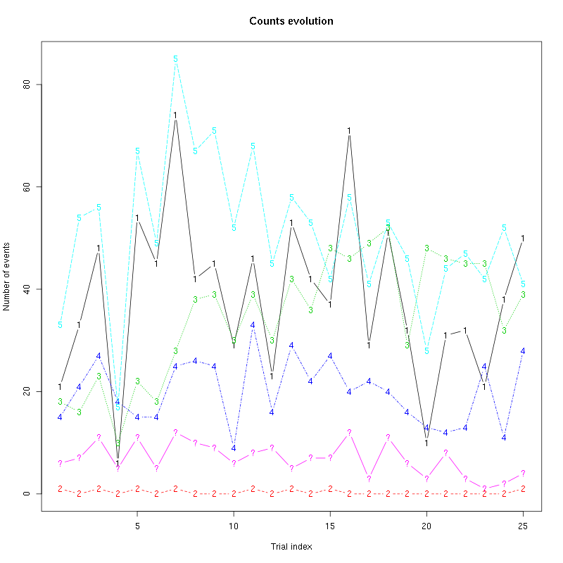
Figure 23: Evolution of the number of events attributed to each unit (1 to 5) or unclassified ("?") during the 25 trials of 1-Hexen-3-ol for tetrodeD1.
The waveform evolution is:
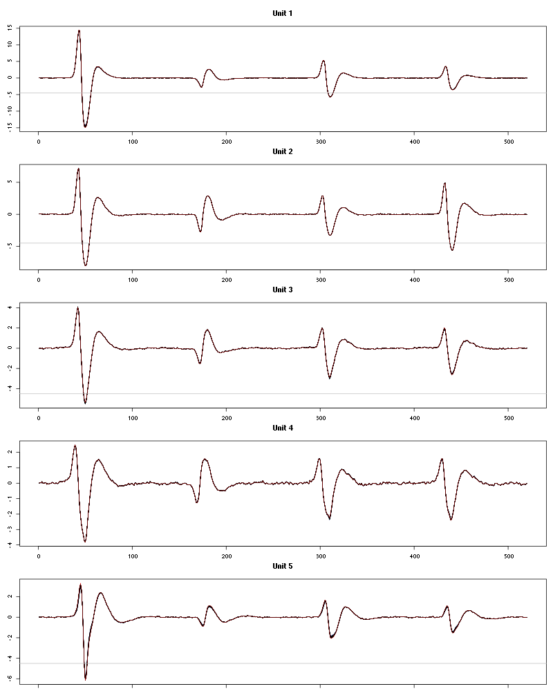
Figure 24: Evolution of the templates of each unit during the 25 trials of 1-Hexen-3-ol for tetrodeD1.
The observed counting processes, inter spike intervals densities and raster plots are:
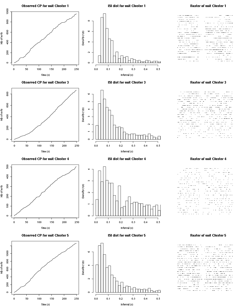
Figure 25: Observed counting processes, empirical inter spike interval distributions and raster plots for 1-Hexen-3-ol.
8.3 Save results
Before analyzing the next set of trials we save the output of sort_many_trials to disk with:
save(a_1_Hexen_3_ol_tetD1,
     file=paste0("tetD1_analysis/tetD1_",stim_name,"_summary_obj.rda"))
We write to disk the spike trains in text mode:
for (c_idx in 1:length(a_1_Hexen_3_ol_tetD1$spike_trains))
    if (!is.null(a_1_Hexen_3_ol_tetD1$spike_trains[[c_idx]]))
        cat(a_1_Hexen_3_ol_tetD1$spike_trains[[c_idx]],
            file=paste0("locust20000421_spike_trains/locust20000421_1-Hexen-3-ol_tetD1_u",
                        c_idx,".txt"),sep="\n")
9 25 trials with 3-Pentanone
We will carry out an analysis of the 25 trials from 3-Pentanone.
9.1 Do the job
stim_name = "3-Pentanone"
a_3_Pentanone_tetD1=smt(stim_name=stim_name,
                        trial_nbs=1:25,
                        centers=a_1_Hexen_3_ol_tetD1$centers,
                        counts=a_1_Hexen_3_ol_tetD1$counts)
9.2 Diagnostic plots
The counts evolution is:
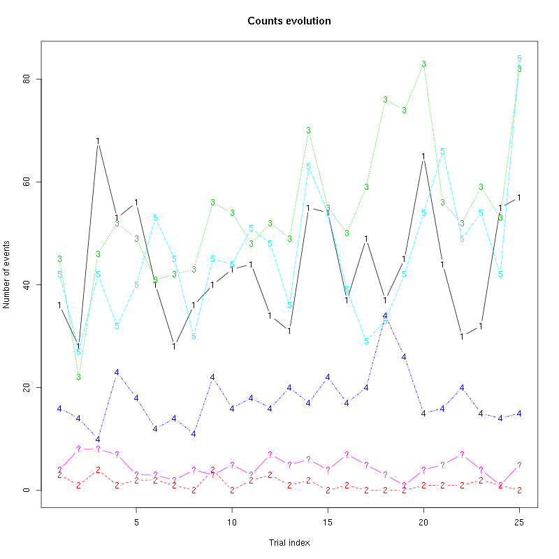
Figure 26: Evolution of the number of events attributed to each unit (1 to 5) or unclassified ("?") during the 25 trials of 3-Pentanone for tetrodeD1.
The waveform evolution is:
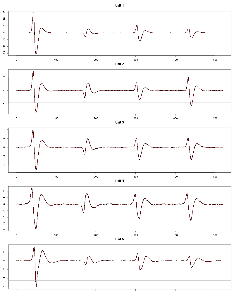
Figure 27: Evolution of the templates of each of the first four units during the 25 trials of 3-Pentanone for tetrodeD1.
The observed counting processes, inter spike intervals densities and raster plots are:
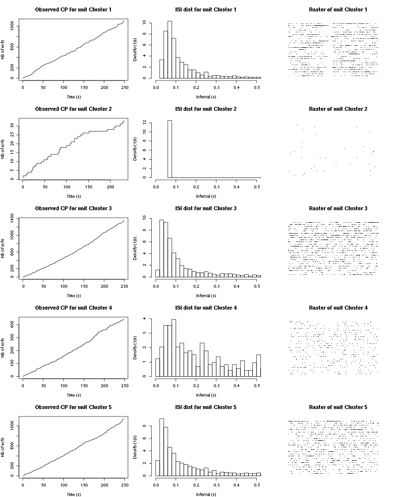
Figure 28: Observed counting processes, empirical inter spike interval distributions and raster plots for 3-Pentanone.
9.3 Save results
Before analyzing the next set of trials we save the output of sort_many_trials to disk with:
save(a_3_Pentanone_tetD1,
     file=paste0("tetD1_analysis/tetD1_",stim_name,"_summary_obj.rda"))
We write to disk the spike trains in text mode:
for (c_idx in 1:length(a_3_Pentanone_tetD1$spike_trains))
    if (!is.null(a_3_Pentanone_tetD1$spike_trains[[c_idx]]))
        cat(a_3_Pentanone_tetD1$spike_trains[[c_idx]],
            file=paste0("locust20000421_spike_trains/locust20000421_3-Pentanone_tetD1_u",
                        c_idx,".txt"),sep="\n")
10 25 trials with 1-Heptanol
We will carry out an analysis of the 25 trials from 1-Heptanol.
10.1 Do the job
stim_name = "1-Heptanol"
a_1_Heptanol_tetD1=smt(stim_name=stim_name,
                       trial_nbs=1:25,
                       centers=a_3_Pentanone_tetD1$centers,
                       counts=a_3_Pentanone_tetD1$counts)
10.2 Diagnostic plots
The counts evolution is:
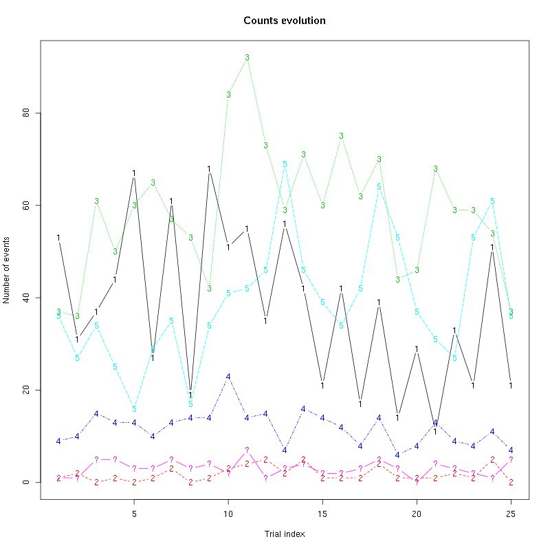
Figure 29: Evolution of the number of events attributed to each unit (1 to 5) or unclassified ("?") during the 25 trials of 1-Heptanol for tetrodeD1.
The waveform evolution is:
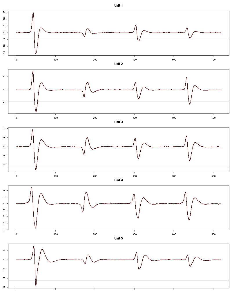
Figure 30: Evolution of the templates of each of the first four units during the 25 trials of 1-Heptanol for tetrodeD1.
The observed counting processes, inter spike intervals densities and raster plots are:
cp_isi_raster(a_1_Heptanol_tetD1)
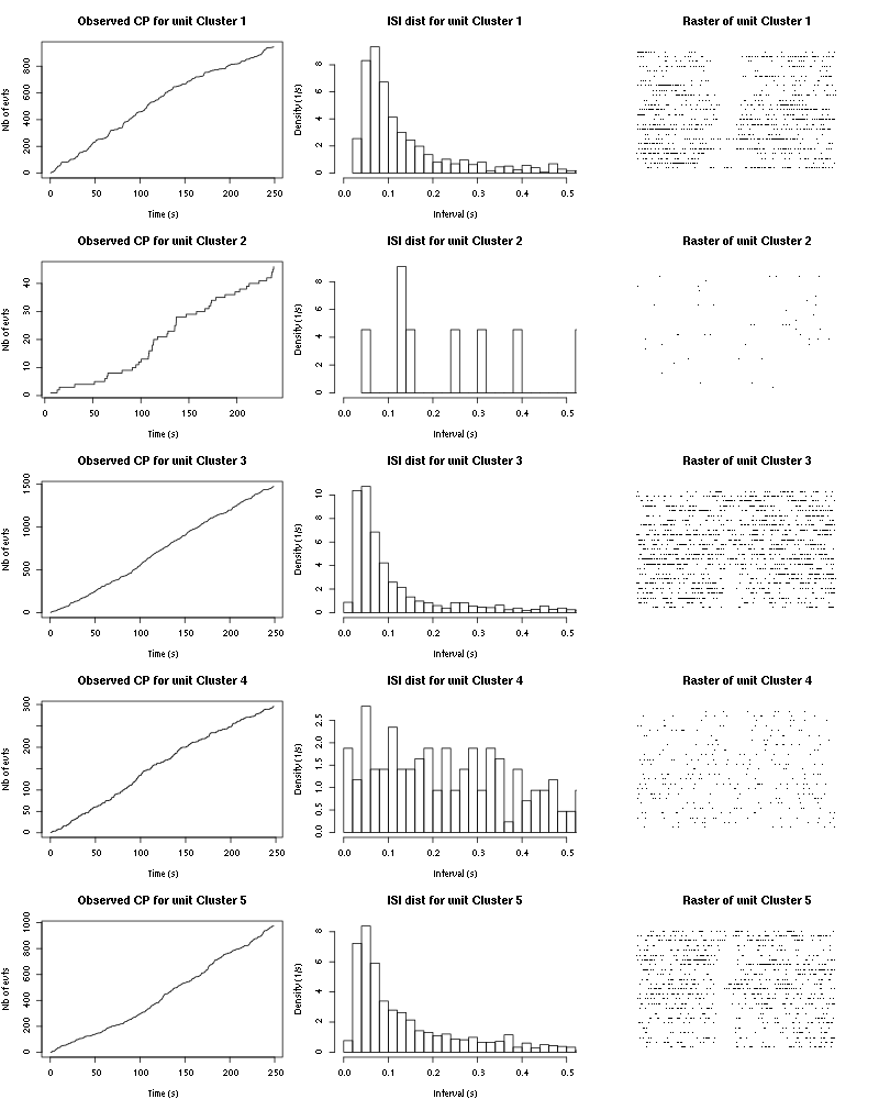
Figure 31: Observed counting processes, empirical inter spike interval distributions and raster plots for 1-Heptanol.
10.3 Save results
Before analyzing the next set of trials we save the output of sort_many_trials to disk with:
save(a_1_Heptanol_tetD1,
     file=paste0("tetD1_analysis/tetD1_",stim_name,"_summary_obj.rda"))
We write to disk the spike trains in text mode:
for (c_idx in 1:length(a_1_Heptanol_tetD1$spike_trains))
    if (!is.null(a_1_Heptanol_tetD1$spike_trains[[c_idx]]))
        cat(a_1_Heptanol_tetD1$spike_trains[[c_idx]],
            file=paste0("locust20000421_spike_trains/locust20000421_1-Heptanol_tetD1_u",
                        c_idx,".txt"),sep="\n")
11 25 trials with 1-Octanol (10^-0) first
We will carry out an analysis of the 25 trials from 1-Octanol (10^-0) first.
11.1 Do the job
stim_name = "1-Octanol (10^-0) first"
a_1_Octanol_0_tetD1=smt(stim_name=stim_name,
                        trial_nbs=1:25,
                        centers=a_1_Heptanol_tetD1$centers,
                        counts=a_1_Heptanol_tetD1$counts)
11.2 Diagnostic plots
The counts evolution is:
 first-count-evolution-tetD1.png)
Figure 32: Evolution of the number of events attributed to each unit (1 to 5) or unclassified ("?") during the 25 trials of 1-Octanol (10^-0) first for tetrodeD1.
The waveform evolution is:
 first-waveform-evolution-tetD1.png)
Figure 33: Evolution of the templates of each of the first four units during the 25 trials of 1-Octanol (10^-0) first for tetrodeD1.
The observed counting processes, inter spike intervals densities and raster plots are:
cp_isi_raster(a_1_Octanol_0_tetD1)
 first-CP-and-ISI-dist-tetD1.png)
Figure 34: Observed counting processes, empirical inter spike interval distributions and raster plots for 1-Octanol (10^-0) first.
11.3 Save results
Before analyzing the next set of trials we save the output of sort_many_trials to disk with:
save(a_1_Octanol_0_tetD1,
     file=paste0("tetD1_analysis/tetD1_",stim_name,"_summary_obj.rda"))
We write to disk the spike trains in text mode:
for (c_idx in 1:length(a_1_Octanol_0_tetD1$spike_trains))
    if (!is.null(a_1_Octanol_0_tetD1$spike_trains[[c_idx]]))
        cat(a_1_Octanol_0_tetD1$spike_trains[[c_idx]],
            file=paste0("locust20000421_spike_trains/locust20000421_1-Octanol (10^-0) first_tetD1_u",
                        c_idx,".txt"),sep="\n")
12 25 trials with 2-Heptanone
We will carry out an analysis of the 25 trials from 2-Heptanone.
12.1 Do the job
stim_name = "2-Heptanone"
a_2_Heptanone_tetD1=smt(stim_name=stim_name,
                        trial_nbs=1:25,
                        centers=a_1_Octanol_0_tetD1$centers,
                        counts=a_1_Octanol_0_tetD1$counts)
12.2 Diagnostic plots
The counts evolution is:
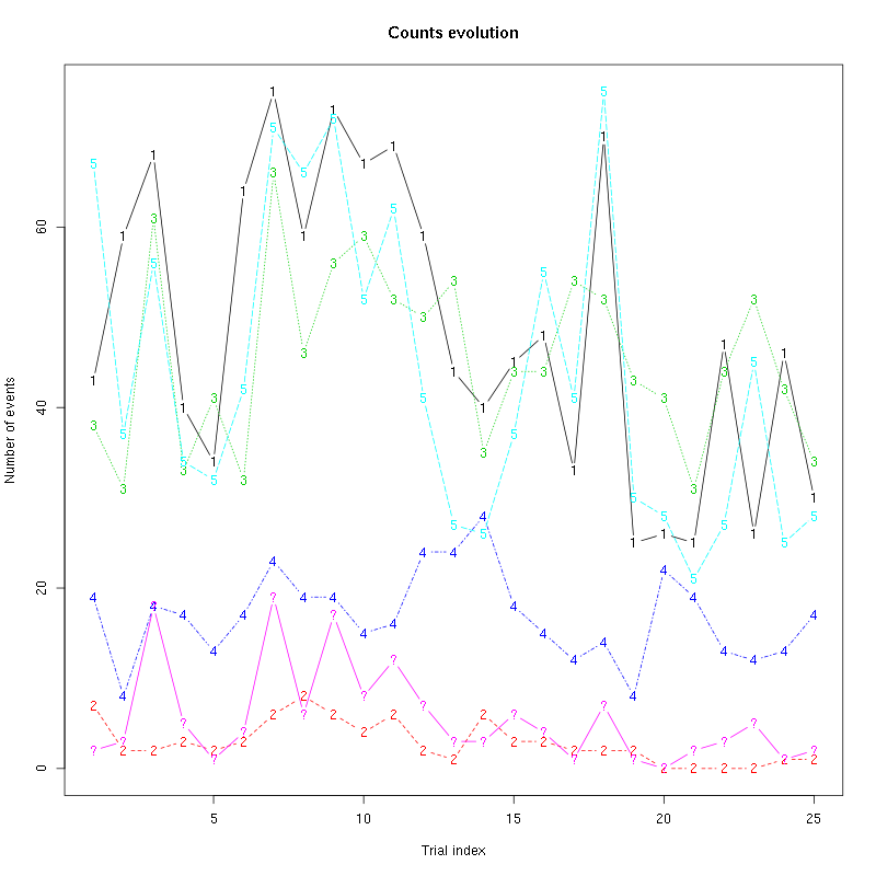
Figure 35: Evolution of the number of events attributed to each unit (1 to 5) or unclassified ("?") during the 25 trials of 2-Heptanone for tetrodeD1.
The waveform evolution is:
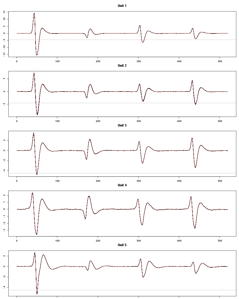
Figure 36: Evolution of the templates of each unit during the 25 trials of 2-Heptanone for tetrodeD1.
The observed counting processes, inter spike intervals densities and raster plots are:
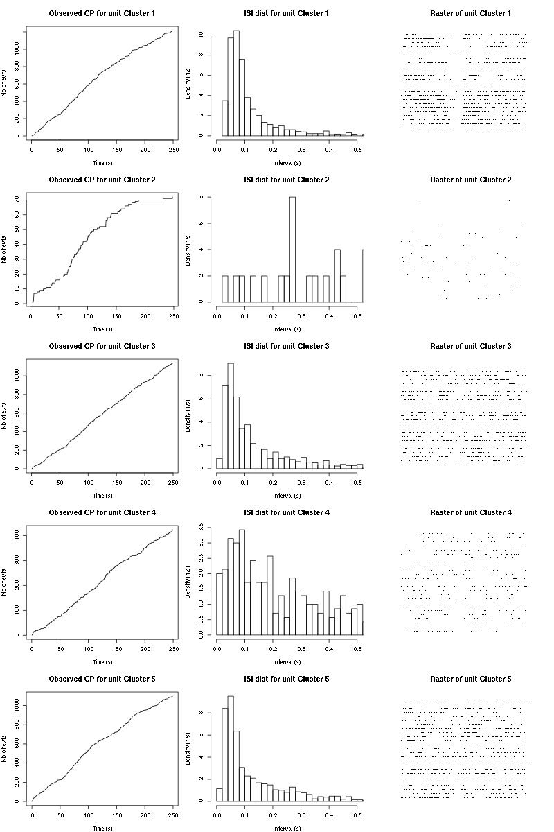
Figure 37: Observed counting processes, empirical inter spike interval distributions and raster plots for 2-Heptanone.
12.3 Save results
Before analyzing the next set of trials we save the output of sort_many_trials to disk with:
save(a_2_Heptanone_tetD1,
     file=paste0("tetD1_analysis/tetD1_",stim_name,"_summary_obj.rda"))
We write to disk the spike trains in text mode:
for (c_idx in 1:length(a_2_Heptanone_tetD1$spike_trains))
    if (!is.null(a_2_Heptanone_tetD1$spike_trains[[c_idx]]))
        cat(a_2_Heptanone_tetD1$spike_trains[[c_idx]],file=paste0("locust20000421_spike_trains/locust20000421_2-Heptanone_tetD1_u",c_idx,".txt"),sep="\n")
13 25 trials with 3-Heptanone
We will carry out an analysis of the 25 trials from 3-Heptanone.
13.1 Do the job
stim_name = "3-Heptanone"
a_3_Heptanone_tetD1=smt(stim_name=stim_name,
                        trial_nbs=1:25,
                        centers=a_2_Heptanone_tetD1$centers,
                        counts=a_2_Heptanone_tetD1$counts)
13.2 Diagnostic plots
The counts evolution is:
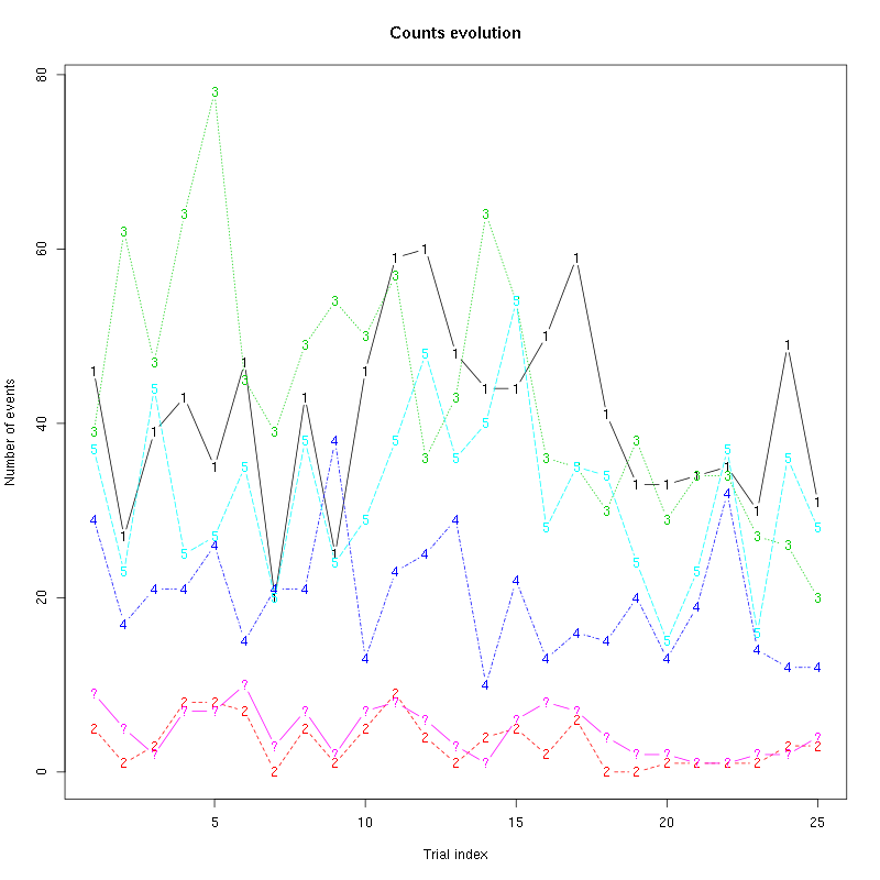
Figure 38: Evolution of the number of events attributed to each unit (1 to 5) or unclassified ("?") during the 25 trials of 3-Heptanone for tetrodeD1.
The waveform evolution is:
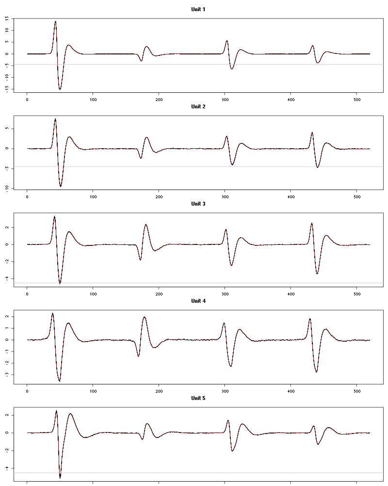
Figure 39: Evolution of the templates of each unit during the 25 trials of 3-Heptanone for tetrodeD1.
The observed counting processes, inter spike intervals densities and raster plots are:
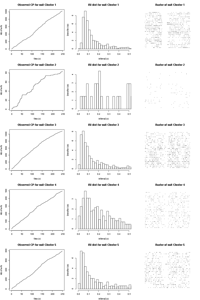
Figure 40: Observed counting processes, empirical inter spike interval distributions and raster plots for 3-Heptanone.
13.3 Save results
Before analyzing the next set of trials we save the output of sort_many_trials to disk with:
save(a_3_Heptanone_tetD1,
     file=paste0("tetD1_analysis/tetD1_",stim_name,"_summary_obj.rda"))
We write to disk the spike trains in text mode:
for (c_idx in 1:length(a_3_Heptanone_tetD1$spike_trains))
    if (!is.null(a_3_Heptanone_tetD1$spike_trains[[c_idx]]))
        cat(a_3_Heptanone_tetD1$spike_trains[[c_idx]],file=paste0("locust20000421_spike_trains/locust20000421_3-Heptanone_tetD1_u",c_idx,".txt"),sep="\n")
14 25 trials with Citral
We will carry out an analysis of the 25 trials from Citral.
14.1 Do the job
stim_name = "Citral"
a_Citral_tetD1=smt(stim_name=stim_name,
                   trial_nbs=1:25,
                   centers=a_3_Heptanone_tetD1$centers,
                   counts=a_3_Heptanone_tetD1$counts)
14.2 Diagnostic plots
The counts evolution is:
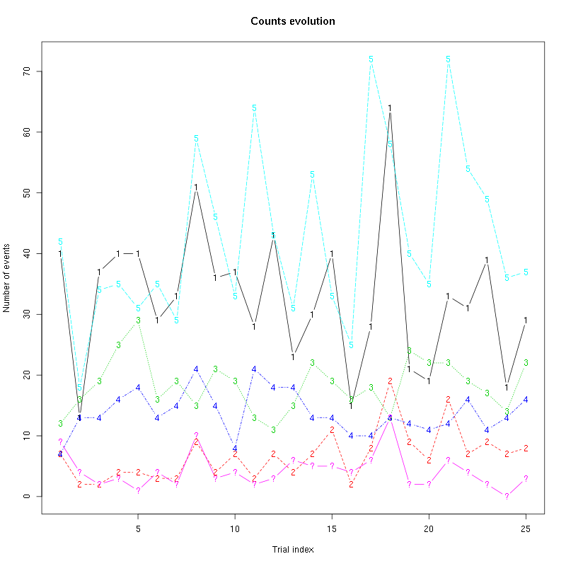
Figure 41: Evolution of the number of events attributed to each unit (1 to 5) or unclassified ("?") during the 25 trials of Citral for tetrodeD1.
The waveform evolution is:
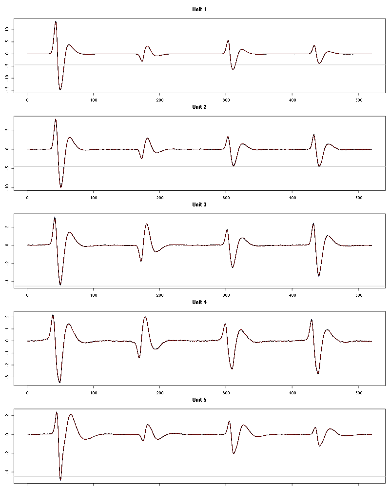
Figure 42: Evolution of the templates of each unit during the 25 trials of Citral for tetrodeD1.
The observed counting processes, inter spike intervals densities and raster plots are:
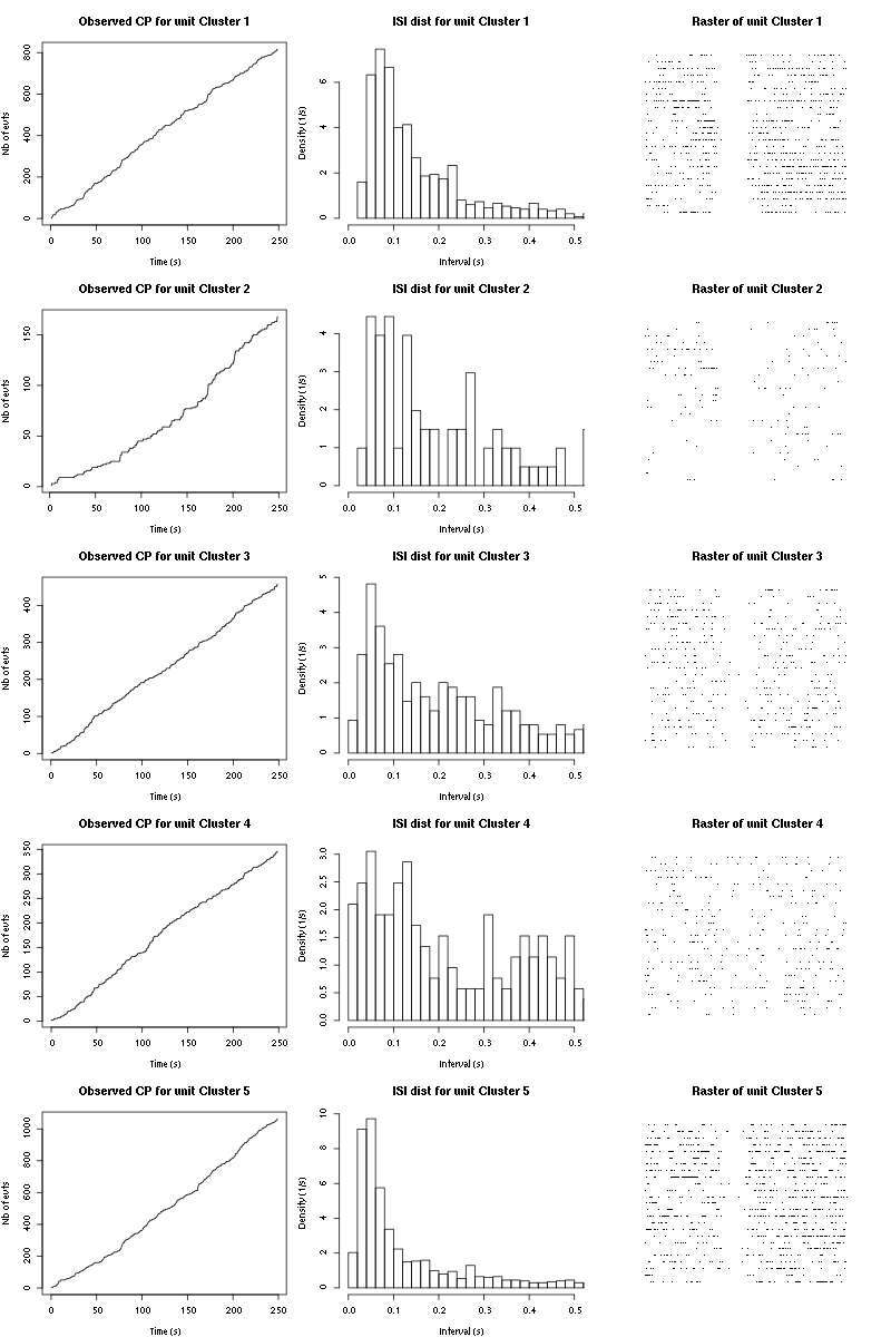
Figure 43: Observed counting processes, empirical inter spike interval distributions and raster plots for Citral.
14.3 Save results
Before analyzing the next set of trials we save the output of sort_many_trials to disk with:
save(a_Citral_tetD1,
     file=paste0("tetD1_analysis/tetD1_",stim_name,"_summary_obj.rda"))
We write to disk the spike trains in text mode:
for (c_idx in 1:length(a_Citral_tetD1$spike_trains))
    if (!is.null(a_Citral_tetD1$spike_trains[[c_idx]]))
        cat(a_Citral_tetD1$spike_trains[[c_idx]],file=paste0("locust20000421_spike_trains/locust20000421_Citral_tetD1_u",c_idx,".txt"),sep="\n")
15 25 trials with Apple
We will carry out an analysis of the 25 trials from Apple.
15.1 Do the job
stim_name = "Apple"
a_Apple_tetD1=smt(stim_name=stim_name,
                  trial_nbs=1:25,
                  centers=a_Citral_tetD1$centers,
                  counts=a_Citral_tetD1$counts)
15.2 Diagnostic plots
The counts evolution is:
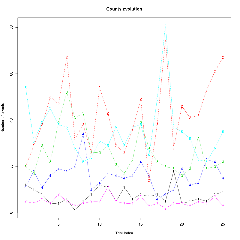
Figure 44: Evolution of the number of events attributed to each unit (1 to 5) or unclassified ("?") during the 25 trials of Apple for tetrodeD1.
The waveform evolution is:
waveform_evolution(a_Apple_tetD1,threshold_factor)
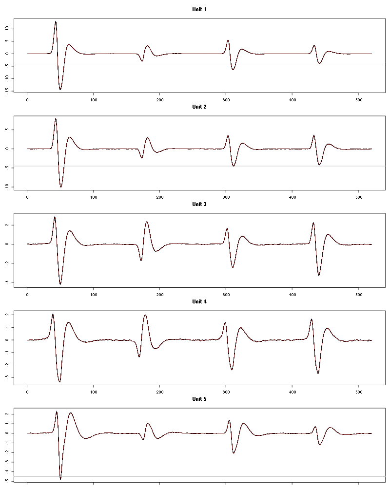
Figure 45: Evolution of the templates of each unit during the 25 trials of Apple for tetrodeD1.
The observed counting processes, inter spike intervals densities and raster plots are:
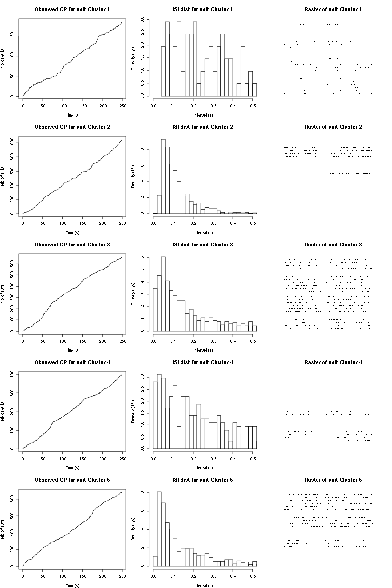
Figure 46: Observed counting processes, empirical inter spike interval distributions and raster plots for Apple.
15.3 Save results
Before analyzing the next set of trials we save the output of sort_many_trials to disk with:
save(a_Apple_tetD1s,
     file=paste0("tetD1_analysis/tetD1_",stim_name,"_summary_obj.rda"))
We write to disk the spike trains in text mode:
for (c_idx in 1:length(a_Apple_tetD1$spike_trains))
    if (!is.null(a_Apple_tetD1$spike_trains[[c_idx]]))
        cat(a_Apple_tetD1$spike_trains[[c_idx]],file=paste0("locust20000421_spike_trains/locust20000421_Apple_tetD1_u",c_idx,".txt"),sep="\n")
16 25 trials with Mint
We will carry out an analysis of the 25 trials from Mint.
16.1 Do the job
stim_name = "Mint"
a_Mint_tetD1=smt(stim_name=stim_name,
                 trial_nbs=1:25,
                 centers=a_Apple_tetD1$centers,
                 counts=a_Apple_tetD1$counts)
16.2 Diagnostic plots
The counts evolution is:
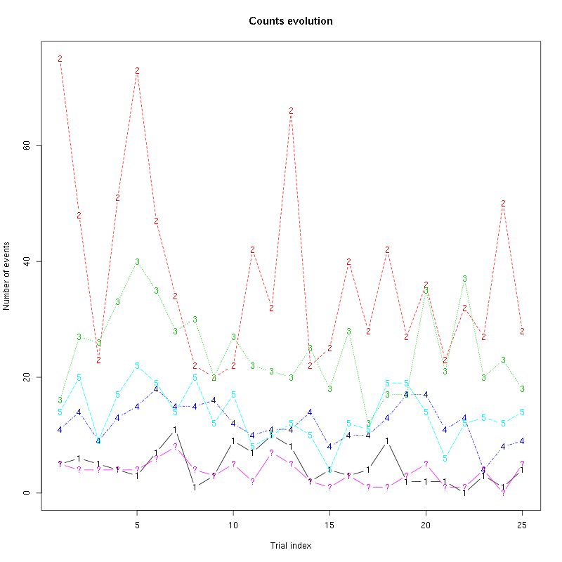
Figure 47: Evolution of the number of events attributed to each unit (1 to 5) or unclassified ("?") during the 25 trials of Mint for tetrodeD1.
The waveform evolution is:
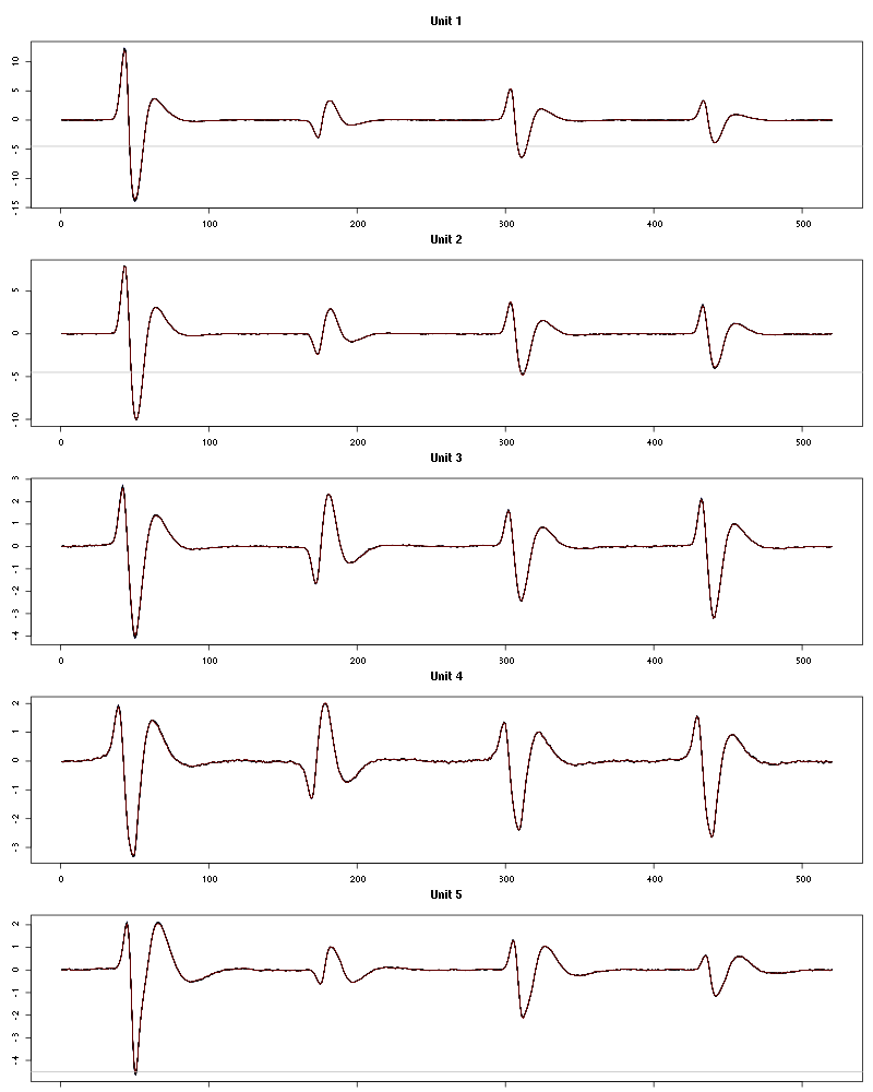
Figure 48: Evolution of the templates of each unit during the 25 trials of Mint for tetrodeD1.
The observed counting processes, inter spike intervals densities and raster plots are:
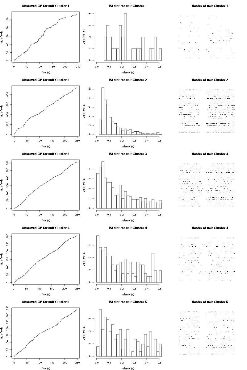
Figure 49: Observed counting processes, empirical inter spike interval distributions and raster plots for Mint.
16.3 Save results
Before analyzing the next set of trials we save the output of sort_many_trials to disk with:
save(a_Mint_tetD1,
     file=paste0("tetD1_analysis/tetD1_",stim_name,"_summary_obj.rda"))
We write to disk the spike trains in text mode:
for (c_idx in 1:length(a_Mint_sterC$spike_trains))
    if (!is.null(a_Mint_sterC$spike_trains[[c_idx]]))
        cat(a_Mint_sterC$spike_trains[[c_idx]],file=paste0("locust20000421_spike_trains/locust20000421_Mint_tetD1_u",c_idx,".txt"),sep="\n")
17 25 trials with Strawberry
We will carry out an analysis of the 25 trials from Strawberry.
17.1 Do the job
stim_name = "Strawberry"
a_Strawberry_tetD1=smt(stim_name=stim_name,
                       trial_nbs=1:25,
                       centers=a_Mint_tetD1$centers,
                       counts=a_Mint_tetD1$counts)
17.2 Diagnostic plots
The counts evolution is:
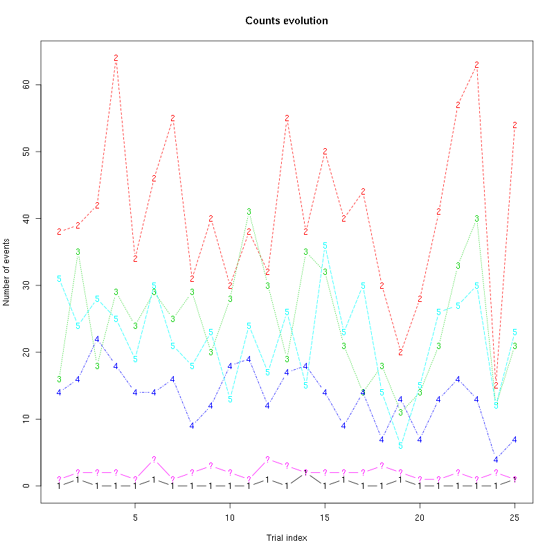
Figure 50: Evolution of the number of events attributed to each unit (1 to 5) or unclassified ("?") during the 25 trials of Strawberry for tetrodeD1.
The waveform evolution is:
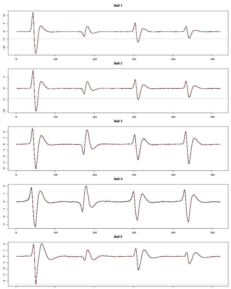
Figure 51: Evolution of the templates of each unit during the 25 trials of Strawberry for tetrodeD1.
The observed counting processes, inter spike intervals densities and raster plots are:
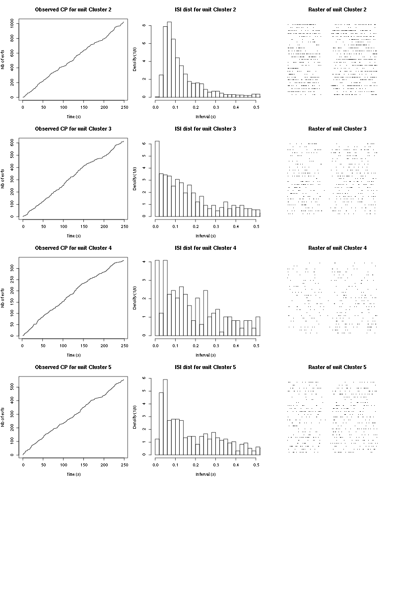
Figure 52: Observed counting processes, empirical inter spike interval distributions and raster plots for Strawberry.
17.3 Save results
Before analyzing the next set of trials we save the output of sort_many_trials to disk with:
save(a_Strawberry_tetD1,
     file=paste0("tetD1_analysis/tetD1_",stim_name,"_summary_obj.rda"))
We write to disk the spike trains in text mode:
for (c_idx in 1:length(a_Strawberry_sterC$spike_trains))
    if (!is.null(a_Strawberry_sterC$spike_trains[[c_idx]]))
        cat(a_Strawberry_sterC$spike_trains[[c_idx]],file=paste0("locust20000421_spike_trains/locust20000421_Strawberry_tetD1_u",c_idx,".txt"),sep="\n")
18 25 trials with Amyl Acetate
We will carry out an analysis of the 25 trials from Amyl Acetate.
18.1 Do the job
stim_name = "Amyl Acetate"
a_Amyl_Acetate_tetD1=smt(stim_name=stim_name,
                         trial_nbs=1:25,
                         centers=a_Strawberry_tetD1$centers,
                         counts=a_Strawberry_tetD1$counts)
18.2 Diagnostic plots
The counts evolution is:
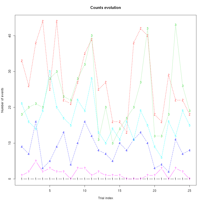
Figure 53: Evolution of the number of events attributed to each unit (1 to 5) or unclassified ("?") during the 25 trials of Amyl Acetate for tetrodeD1.
The waveform evolution is:
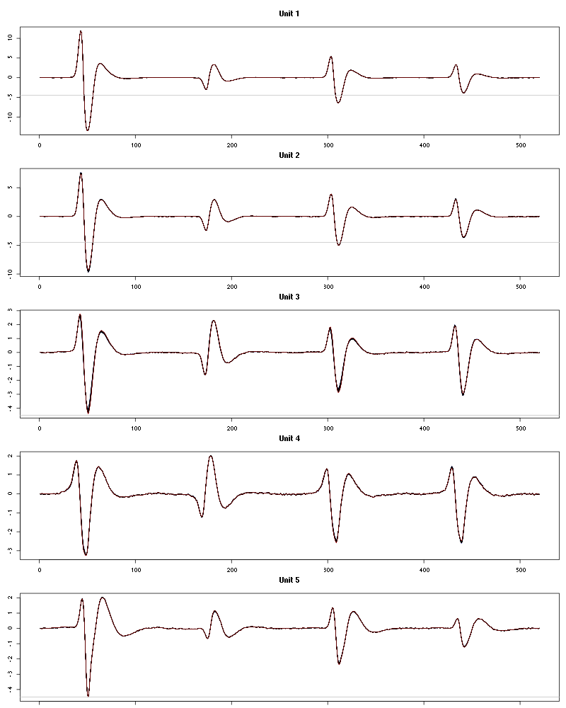
Figure 54: Evolution of the templates of each unit during the 25 trials of Amyl Acetate for tetrodeD1.
The observed counting processes, inter spike intervals densities and raster plots are:
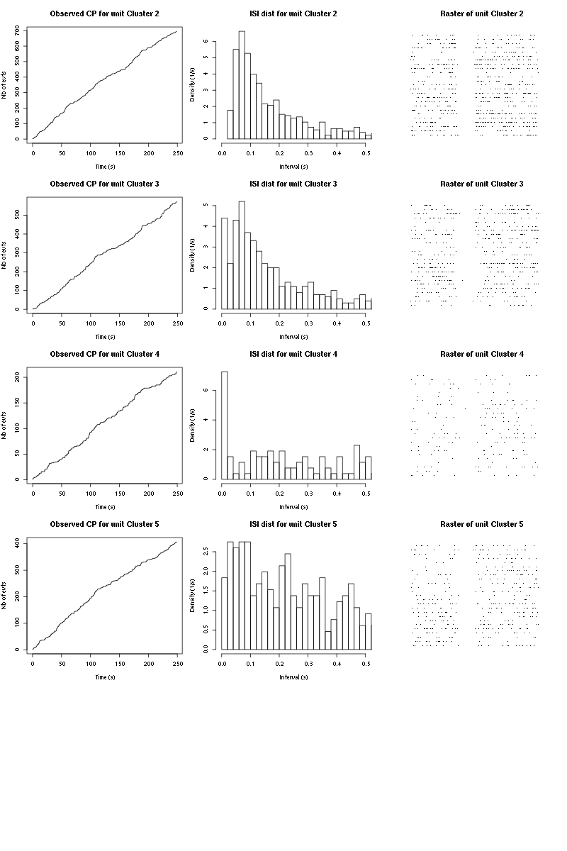
Figure 55: Observed counting processes, empirical inter spike interval distributions and raster plots for Amyl Acetate.
18.3 Save results
Before analyzing the next set of trials we save the output of sort_many_trials to disk with:
save(a_Amyl_Acetate_tetD1,
     file=paste0("tetD1_analysis/tetD1_",stim_name,"_summary_obj.rda"))
We write to disk the spike trains in text mode:
for (c_idx in 1:length(a_Amyl_Acetate_tetD1$spike_trains))
    if (!is.null(a_Amyl_Acetate_tetD1$spike_trains[[c_idx]]))
        cat(a_Amyl_Acetate_tetD1$spike_trains[[c_idx]],file=paste0("locust20000421_spike_trains/locust20000421_Amyl Acetate_tetD1_u",c_idx,".txt"),sep="\n")
19 25 trials with Octaldehyde
We will carry out an analysis of the 25 trials from Octaldehyde.
19.1 Do the job
stim_name = "Octaldehyde"
a_Octaldehyde_tetD1=smt(stim_name=stim_name,
                        trial_nbs=1:25,
                        centers=a_Amyl_Acetate_tetD1$centers,
                        counts=a_Amyl_Acetate_tetD1$counts)
19.2 Diagnostic plots
The counts evolution is:
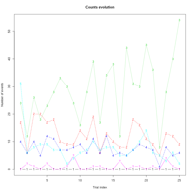
Figure 56: Evolution of the number of events attributed to each unit (1 to 5) or unclassified ("?") during the 25 trials of Octaldehyde for tetrodeD1.
The waveform evolution is:
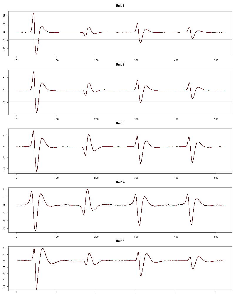
Figure 57: Evolution of the templates of each unit during the 25 trials of Octaldehyde for tetrodeD1.
The observed counting processes, inter spike intervals densities and raster plots are:
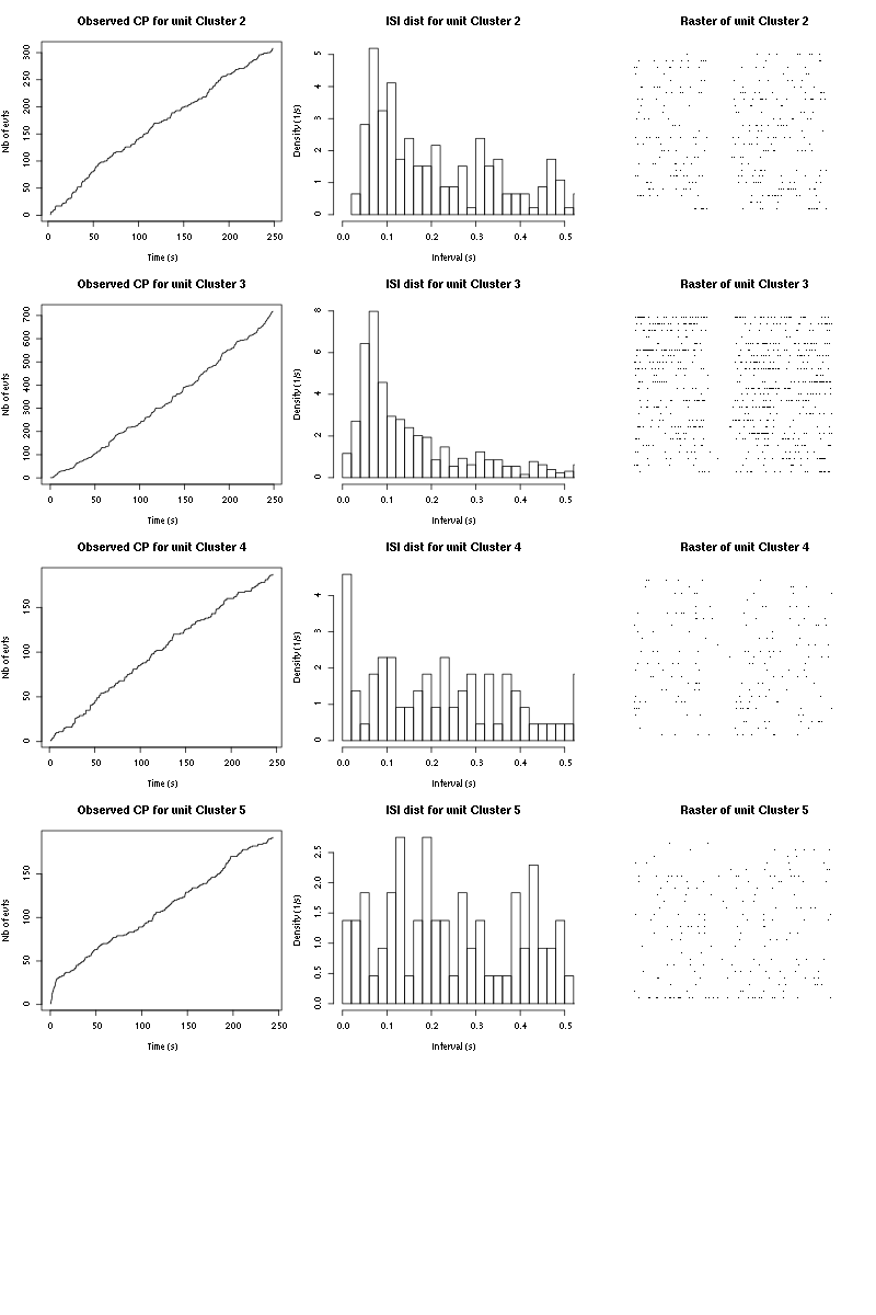
Figure 58: Observed counting processes, empirical inter spike interval distributions and raster plots for Octaldehyde.
19.3 Save results
Before analyzing the next set of trials we save the output of sort_many_trials to disk with:
save(a_Octaldehyde_tetD1,
     file=paste0("tetD1_analysis/tetD1_",stim_name,"_summary_obj.rda"))
We write to disk the spike trains in text mode:
for (c_idx in 1:length(a_Octaldehyde_tetD1$spike_trains))
    if (!is.null(a_Octaldehyde_tetD1$spike_trains[[c_idx]]))
        cat(a_Octaldehyde_tetD1$spike_trains[[c_idx]],file=paste0("locust20000421_spike_trains/locust20000421_Octaldehyde_tetD1_u",c_idx,".txt"),sep="\n")
20 25 trials with 1-Octanol (10^-5)
We will carry out an analysis of the 25 trials from 1-Octanol (10^-5).
20.1 Do the job
stim_name = "1-Octanol (10^-5)"
a_1_Octanol_5_tetD1=smt(stim_name=stim_name,
                        trial_nbs=1:25,
                        centers=a_Octaldehyde_tetD1$centers,
                        counts=a_Octaldehyde_tetD1$counts)
20.2 Diagnostic plots
The counts evolution is:
-count-evolution-tetD1.png)
Figure 59: Evolution of the number of events attributed to each unit (1 to 5) or unclassified ("?") during the 25 trials of 1-Octanol (10^-5) for tetrodeD1.
The waveform evolution is:
-waveform-evolution-tetD1.png)
Figure 60: Evolution of the templates of each unit during the 25 trials of 1-Octanol (10^-5) for tetrodeD1.
The observed counting processes, inter spike intervals densities and raster plots are:
-CP-and-ISI-dist-tetD1.png)
Figure 61: Observed counting processes, empirical inter spike interval distributions and raster plots for 1-Octanol (10^-5).
20.3 Save results
Before analyzing the next set of trials we save the output of sort_many_trials to disk with:
save(a_1_Octanol_5_tetD1,
     file=paste0("tetD1_analysis/tetD1_",stim_name,"_summary_obj.rda"))
We write to disk the spike trains in text mode:
for (c_idx in 1:length(a_1_Octanol_5_tetD1$spike_trains))
    if (!is.null(a_1_Octanol_5_tetD1$spike_trains[[c_idx]]))
        cat(a_1_Octanol_5_tetD1$spike_trains[[c_idx]],file=paste0("locust20000421_spike_trains/locust20000421_1-Octanol (10^-5)_tetD1_u",c_idx,".txt"),sep="\n")
21 25 trials with 1-Octanol (10^-4)
We will carry out an analysis of the 25 trials from 1-Octanol (10^-4).
21.1 Do the job
stim_name = "1-Octanol (10^-4)"
a_1_Octanol_4_tetD1=smt(stim_name=stim_name,
                        trial_nbs=1:25,
                        centers=a_1_Octanol_5_tetD1$centers,
                        counts=a_1_Octanol_5_tetD1$counts)
21.2 Diagnostic plots
The counts evolution is:
-count-evolution-tetD1.png)
Figure 62: Evolution of the number of events attributed to each unit (1 to 5) or unclassified ("?") during the 25 trials of 1-Octanol (10^-4) for tetrodeD1.
The waveform evolution is:
-waveform-evolution-tetD1.png)
Figure 63: Evolution of the templates of each unit during the 25 trials of 1-Octanol (10^-4) for tetrodeD1.
The observed counting processes, inter spike intervals densities and raster plots are:
-CP-and-ISI-dist-tetD1.png)
Figure 64: Observed counting processes, empirical inter spike interval distributions and raster plots for 1-Octanol (10^-4).
21.3 Save results
Before analyzing the next set of trials we save the output of sort_many_trials to disk with:
save(a_1_Octanol_4_tetD1,
     file=paste0("tetD1_analysis/tetD1_",stim_name,"_summary_obj.rda"))
We write to disk the spike trains in text mode:
for (c_idx in 1:length(a_1_Octanol_4_tetD1$spike_trains))
    if (!is.null(a_1_Octanol_4_tetD1$spike_trains[[c_idx]]))
        cat(a_1_Octanol_4_tetD1$spike_trains[[c_idx]],file=paste0("locust20000421_spike_trains/locust20000421_1-Octanol (10^-4)_tetD1_u",c_idx,".txt"),sep="\n")
22 25 trials with 1-Octanol (10^-3)
We will carry out an analysis of the 25 trials from 1-Octanol (10^-3).
22.1 Do the job
stim_name = "1-Octanol (10^-3)"
a_1_Octanol_3_tetD1=smt(stim_name=stim_name,
                        trial_nbs=1:25,
                        centers=a_1_Octanol_4_tetD1$centers,
                        counts=a_1_Octanol_4_tetD1$counts)
22.2 Diagnostic plots
The counts evolution is:
-count-evolution-tetD1.png)
Figure 65: Evolution of the number of events attributed to each unit (1 to 5) or unclassified ("?") during the 25 trials of 1-Octanol (10^-3) for tetrodeD1.
The waveform evolution is:
-waveform-evolution-tetD1.png)
Figure 66: Evolution of the templates of each unit during the 25 trials of 1-Octanol (10^-3) for tetrodeD1.
The observed counting processes, inter spike intervals densities and raster plots are:
-CP-and-ISI-dist-tetD1.png)
Figure 67: Observed counting processes, empirical inter spike interval distributions and raster plots for 1-Octanol (10^-3).
22.3 Save results
Before analyzing the next set of trials we save the output of sort_many_trials to disk with:
save(a_1_Octanol_3_tetD1,
     file=paste0("tetD1_analysis/tetD1_",stim_name,"_summary_obj.rda"))
We write to disk the spike trains in text mode:
for (c_idx in 1:length(a_1_Octanol_3_tetD1$spike_trains))
    if (!is.null(a_1_Octanol_3_tetD1$spike_trains[[c_idx]]))
        cat(a_1_Octanol_3_tetD1$spike_trains[[c_idx]],file=paste0("locust20000421_spike_trains/locust20000421_1-Octanol (10^-3)_tetD1_u",c_idx,".txt"),sep="\n")
23 25 trials with 1-Octanol (10^-2)
We will carry out an analysis of the 25 trials from 1-Octanol (10^-2).
23.1 Do the job
stim_name = "1-Octanol (10^-2)"
a_1_Octanol_2_tetD1=smt(stim_name=stim_name,
                        trial_nbs=1:25,
                        centers=a_1_Octanol_3_tetD1$centers,
                        counts=a_1_Octanol_3_tetD1$counts)
23.2 Diagnostic plots
The counts evolution is:
-count-evolution-tetD1.png)
Figure 68: Evolution of the number of events attributed to each unit (1 to 5) or unclassified ("?") during the 25 trials of 1-Octanol (10^-2) for tetrodeD1.
The waveform evolution is:
-waveform-evolution-tetD1.png)
Figure 69: Evolution of the templates of each unit during the 25 trials of 1-Octanol (10^-2) for tetrodeD1.
The observed counting processes, inter spike intervals densities and raster plots are:
-CP-and-ISI-dist-tetD1.png)
Figure 70: Observed counting processes, empirical inter spike interval distributions and raster plots for 1-Octanol (10^-2).
23.3 Save results
Before analyzing the next set of trials we save the output of sort_many_trials to disk with:
save(a_1_Octanol_2_tetD1,
     file=paste0("tetD1_analysis/tetD1_",stim_name,"_summary_obj.rda"))
We write to disk the spike trains in text mode:
for (c_idx in 1:length(a_1_Octanol_2_tetD1$spike_trains))
    if (!is.null(a_1_Octanol_2_tetD1$spike_trains[[c_idx]]))
        cat(a_1_Octanol_2_tetD1$spike_trains[[c_idx]],file=paste0("locust20000421_spike_trains/locust20000421_1-Octanol (10^-2)_tetD1_u",c_idx,".txt"),sep="\n")
24 25 trials with 1-Octanol (10^-1)
We will carry out an analysis of the 25 trials from 1-Octanol (10^-1).
24.1 Do the job
stim_name = "1-Octanol (10^-1)"
a_1_Octanol_1_tetD1=smt(stim_name=stim_name,
                        trial_nbs=1:25,
                        centers=a_1_Octanol_2_tetD1$centers,
                        counts=a_1_Octanol_2_tetD1$counts)
24.2 Diagnostic plots
The counts evolution is:
-count-evolution-tetD1.png)
Figure 71: Evolution of the number of events attributed to each unit (1 to 5) or unclassified ("?") during the 25 trials of 1-Octanol (10^-1) for tetrodeD1.
The waveform evolution is:
-waveform-evolution-tetD1.png)
Figure 72: Evolution of the templates of each unit during the 25 trials of 1-Octanol (10^-1) for tetrodeD1.
The observed counting processes, inter spike intervals densities and raster plots are:
-CP-and-ISI-dist-tetD1.png)
Figure 73: Observed counting processes, empirical inter spike interval distributions and raster plots for 1-Octanol (10^-1).
24.3 Save results
Before analyzing the next set of trials we save the output of sort_many_trials to disk with:
save(a_1_Octanol_1_tetD1,
     file=paste0("tetD1_analysis/tetD1_",stim_name,"_summary_obj.rda"))
We write to disk the spike trains in text mode:
for (c_idx in 1:length(a_1_Octanol_1_tetD1$spike_trains))
    if (!is.null(a_1_Octanol_1_tetD1$spike_trains[[c_idx]]))
        cat(a_1_Octanol_1_tetD1$spike_trains[[c_idx]],file=paste0("locust20000421_spike_trains/locust20000421_1-Octanol (10^-1)_tetD1_u",c_idx,".txt"),sep="\n")
25 25 trials with 1-Octanol (10^-0) second
We will carry out an analysis of the 25 trials from 1-Octanol (10^-0) second.
25.1 Do the job
stim_name = "1-Octanol (10^-0) second"
a_1_Octanol_0b_tetD1=smt(stim_name=stim_name,
                         trial_nbs=1:25,
                         centers=a_1_Octanol_1_tetD1$centers,
                         counts=a_1_Octanol_1_tetD1$counts)
25.2 Diagnostic plots
The counts evolution is:
 second-count-evolution-tetD1.png)
Figure 74: Evolution of the number of events attributed to each unit (1 to 5) or unclassified ("?") during the 25 trials of 1-Octanol (10^-0) second for tetrodeD1.
The waveform evolution is:
 second-waveform-evolution-tetD1.png)
Figure 75: Evolution of the templates of each unit during the 25 trials of 1-Octanol (10^-0) second for tetrodeD1.
The observed counting processes, inter spike intervals densities and raster plots are:
 second-CP-and-ISI-dist-tetD1.png)
Figure 76: Observed counting processes, empirical inter spike interval distributions and raster plots for 1-Octanol (10^-0) second.
25.3 Save results
Before analyzing the next set of trials we save the output of sort_many_trials to disk with:
save(a_1_Octanol_0b_tetD1,
     file=paste0("tetD1_analysis/tetD1_",stim_name,"_summary_obj.rda"))
We write to disk the spike trains in text mode:
for (c_idx in 1:length(a_1_Octanol_0b_tetD1$spike_trains))
    if (!is.null(a_1_Octanol_0b_tetD1$spike_trains[[c_idx]]))
        cat(a_1_Octanol_0b_tetD1$spike_trains[[c_idx]],file=paste0("locust20000421_spike_trains/locust20000421_1-Octanol (10^-0) second_tetD1_u",c_idx,".txt"),sep="\n")