Sorting data set 20000421 tetrode D2 (channels 13, 14, 15, 16)
Table of Contents
- 1. Introduction
- 2. Tetrode D2 (channels 13, 14, 15, 16) analysis
- 2.1. Loading the data
- 2.2. Five number summary
- 2.3. Plot the data
- 2.4. Data normalization
- 2.5. Spike detection
- 2.6. Cuts
- 2.7. Events
- 2.8. Removing obvious superposition
- 2.9. Dimension reduction
- 2.10. Exporting for
GGobi - 2.11. kmeans clustering with 5 and 4 clusters
- 2.12. Long cuts creation
- 2.13. Peeling
- 2.14. Getting the spike trains
- 2.15. Getting the inter spike intervals and the forward and backward recurrence times
- 2.16. Testing "all at once"
- 3. Analyzing a sequence of trials
- 4. Systematic analysis of the 30 trials from
1-Hexanol - 5. 25 trials with
Hexanal - 6. 25 trials with
Cis-3-Hexen-1-ol - 7. 25 trials with
Trans-2-Hexen-1-ol - 8. 25 trials with
1-Hexen-3-ol - 9. 25 trials with
3-Pentanone - 10. 25 trials with
1-Heptanol - 11. 25 trials with
1-Octanol (10^-0) first - 12. 25 trials with
2-Heptanone - 13. 25 trials with
3-Heptanone - 14. 25 trials with
Citral - 15. 25 trials with
Apple - 16. 25 trials with
Mint - 17. 25 trials with
Strawberry - 18. 25 trials with
Amyl Acetate - 19. 25 trials with
Octaldehyde - 20. 25 trials with
1-Octanol (10^-5) - 21. 25 trials with
1-Octanol (10^-4) - 22. 25 trials with
1-Octanol (10^-3) - 23. 25 trials with
1-Octanol (10^-2) - 24. 25 trials with
1-Octanol (10^-1) - 25. 25 trials with
1-Octanol (10^-0) second
1 Introduction
This is the description of how to do the (spike) sorting of tetrode D2 (channels 13, 14, 15, 16) from data set locust20000421.
1.1 Getting the data
The data are in file locust20000421.hdf5 located on zenodo and can be downloaded interactivelly with a web browser or by typing at the command line:
wget https://zenodo.org/record/21589/files/locust20000421.hdf5
In the sequel I will assume that R has been started in the directory where the data were downloaded (in other words, the working direcory should be the one containing the data.
The data are in HDF5 format and the easiest way to get them into R is to install the rhdf5 package from Bioconductor. Once the installation is done, the library is loaded into R with:
library(rhdf5)
We can then get a (long and detailed) listing of our data file content with (result not shown):
h5ls("locust20000421.hdf5")
We can get the content of LabBook metadata from the shell with:
h5dump -a "LabBook" locust20000421.hdf5
1.2 Getting the code
The code can be sourced as follows:
source("https://raw.githubusercontent.com/christophe-pouzat/zenodo-locust-datasets-analysis/master/R_Sorting_Code/sorting_with_r.R")
2 Tetrode D2 (channels 13, 14, 15, 16) analysis
We now want to get our "model", that is a dictionnary of waveforms (one waveform per neuron and per recording site). To that end we are going to use the first 60 s of data contained in the Spontaneous Group (in HDF5 jargon).
2.1 Loading the data
So we start by loading the data from channels 13, 14, 15, 16 into R:
lD = rbind(cbind(h5read("locust20000421.hdf5", "/Spontaneous/ch13"),
                 h5read("locust20000421.hdf5", "/Spontaneous/ch14"),
                 h5read("locust20000421.hdf5", "/Spontaneous/ch15"),
                 h5read("locust20000421.hdf5", "/Spontaneous/ch16")))
dim(lD)
| 892928 |
| 4 |
2.2 Five number summary
We get the Five number summary with:
summary(lD,digits=2)
| Min. :1541 | Min. :1462 | Min. :1267 | Min. :1670 |
| 1st Qu.:2008 | 1st Qu.:2005 | 1st Qu.:2022 | 1st Qu.:2023 |
| Median :2047 | Median :2049 | Median :2065 | Median :2063 |
| Mean :2046 | Mean :2048 | Mean :2063 | Mean :2063 |
| 3rd Qu.:2085 | 3rd Qu.:2092 | 3rd Qu.:2106 | 3rd Qu.:2103 |
| Max. :2498 | Max. :2480 | Max. :2612 | Max. :2392 |
It shows that the channels have very similar properties as far as the median and the inter-quartile range (IQR) are concerned. The minimum is much smaller on the third channel. This suggests that the largest spikes are going to be found here (remember that spikes are going mainly downwards).
2.3 Plot the data
We "convert" the data matrix lD into a time series object with:
lD = ts(lD,start=0,freq=15e3)
We can then plot the whole data with (not shown since it makes a very figure):
plot(lD)
2.4 Data normalization
As always we normalize such that the median absolute deviation (MAD) becomes 1:
lD.mad = apply(lD,2,mad)
lD = t((t(lD)-apply(lD,2,median))/lD.mad)
lD = ts(lD,start=0,freq=15e3)
Once this is done we explore interactively the data with:
explore(lD,col=c("black","grey70"))
Most spikes can be seen on the 4 recording sites and there are different spike waveform!
2.5 Spike detection
Since the spikes are mainly going downwards, we will detect valleys instead of peaks:
lDf = -lD
filter_length = 3
threshold_factor = 5
lDf = filter(lDf,rep(1,filter_length)/filter_length)
lDf[is.na(lDf)] = 0
lDf.mad = apply(lDf,2,mad)
lDf_mad_original = lDf.mad
lDf = t(t(lDf)/lDf_mad_original)
thrs = threshold_factor*c(1,1,1,1)
bellow.thrs = t(t(lDf) < thrs)
lDfr = lDf
lDfr[bellow.thrs] = 0
remove(lDf)
sp0 = peaks(apply(lDfr,1,sum),15)
remove(lDfr)
sp0
eventsPos object with indexes of 1615 events.
  Mean inter event interval: 551.86 sampling points, corresponding SD: 584.61 sampling points
  Smallest and largest inter event intervals: 17 and 6721 sampling points.
Every time a filter length / threshold combination is tried, the detection is checked interactively with:
explore(sp0,lD,col=c("black","grey50"))
2.6 Cuts
We proceed as usual to get the cut length right:
evts = mkEvents(sp0,lD,49,50)
evts.med = median(evts)
evts.mad = apply(evts,1,mad)
plot_range = range(c(evts.med,evts.mad))
plot(evts.med,type="n",ylab="Amplitude",
     ylim=plot_range)
abline(v=seq(0,400,10),col="grey")
abline(h=c(0,1),col="grey")
lines(evts.med,lwd=2)
lines(evts.mad,col=2,lwd=2)
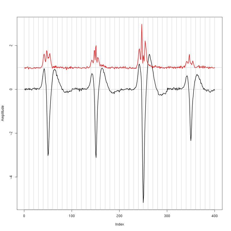
Figure 1: Setting the cut length for the data from tetrode D2 (channels 13, 14, 15, 16). We see that we need 15 points before the peak and 20 after.
We see that we need roughly 15 points before the peak and 20 after.
2.7 Events
We now cut our events:
evts = mkEvents(sp0,lD,14,20)
summary(evts)
events object deriving from data set: lD.
 Events defined as cuts of 35 sampling points on each of the 4 recording sites.
 The 'reference' time of each event is located at point 15 of the cut.
 There are 1615 events in the object.
We can as usual visualize the first 200 events with:
evts[,1:200]
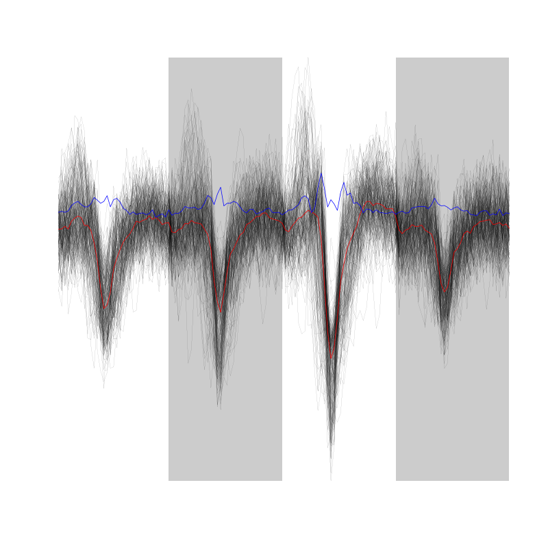
Figure 2: First 200 events for the data from tetrode D2 (channels 1, 3, 5, 7).
There are few superpositions so we try to remove the most obvious ones before doing the dimension reduction.
2.8 Removing obvious superposition
Since some spikes have a pronounced early peak, we will look for superposition only on the late phase (last 10 points) of the events. We define function goodEvtsFct with:
goodEvtsFct = function(samp,thr=3) {
    samp.med = apply(samp,1,median)
    samp.mad = apply(samp,1,mad)
    samp.r = apply(samp,2,function(x) {x[1:25] = 0;x})
    apply(samp.r,2,function(x) all(abs(x-samp.med) < thr*samp.mad))
}
We apply it with a threshold of 5 times the MAD:
goodEvts = goodEvtsFct(evts,5)
2.9 Dimension reduction
We do a PCA on our good events set:
evts.pc = prcomp(t(evts[,goodEvts]))
We look at the projections on the first 4 principle components:
panel.dens = function(x,...) {
  usr = par("usr")
  on.exit(par(usr))
  par(usr = c(usr[1:2], 0, 1.5) )
  d = density(x, adjust=0.5)
  x = d$x
  y = d$y
  y = y/max(y)
  lines(x, y, col="grey50", ...)
}
pairs(evts.pc$x[,1:4],pch=".",gap=0,diag.panel=panel.dens)
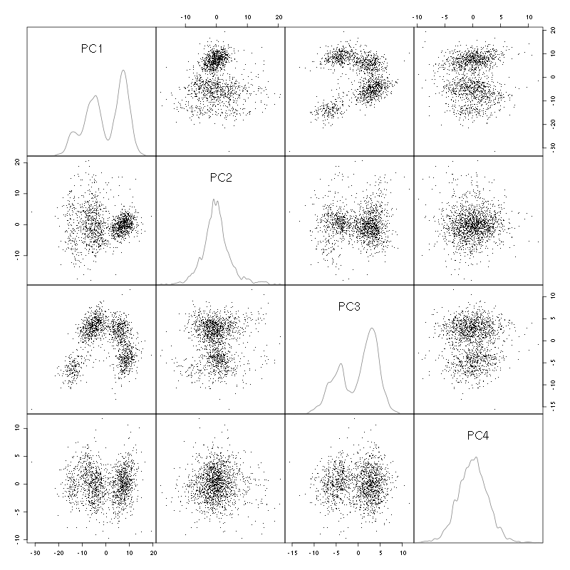
Figure 3: Events from tetrode D2 (channels 13, 14, 15, 16) projected onto the first 4 PCs.
I see at least 4 clusters. We can also look at the projections on the PC pairs defined by the next 4 PCs:
pairs(evts.pc$x[,5:8],pch=".",gap=0,diag.panel=panel.dens)
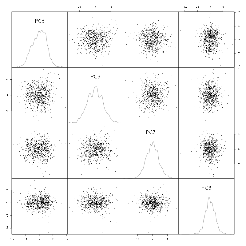
Figure 4: Events from tetrode D2 (channels 13, 14, 15, 16) projected onto PC 5 to 8.
There is not much structure left beyond the 4th PC.
2.10 Exporting for GGobi
We export the events projected onto the first 8 principle components in csv format:
write.csv(evts.pc$x[,1:8],file="tetD2_evts.csv")
Using the rotation display of GGobi with the first 3 principle components and the 2D tour with the first 4 components I see at least 4 clusters but there are probably 5 or 6. So we will start with a kmeans with 5 centers.
2.11 kmeans clustering with 5 and 4 clusters
nbc=5
set.seed(20110928,kind="Mersenne-Twister")
km = kmeans(evts.pc$x[,1:4],centers=nbc,iter.max=100,nstart=100)
label = km$cluster
cluster.med = sapply(1:nbc, function(cIdx) median(evts[,goodEvts][,label==cIdx]))
sizeC = sapply(1:nbc,function(cIdx) sum(abs(cluster.med[,cIdx])))
newOrder = sort.int(sizeC,decreasing=TRUE,index.return=TRUE)$ix
cluster.mad = sapply(1:nbc, function(cIdx) {ce = t(evts[,goodEvts]);ce = ce[label==cIdx,];apply(ce,2,mad)})
cluster.med = cluster.med[,newOrder]
cluster.mad = cluster.mad[,newOrder]
labelb = sapply(1:nbc, function(idx) (1:nbc)[newOrder==idx])[label]
We write a new csv file with the data and the labels:
write.csv(cbind(evts.pc$x[,1:4],labelb),file="tetD2_sorted.csv")
It gives what was expected.
We get a plot showing the events attributed to each unit with:
layout(matrix(1:nbc,nr=nbc))
par(mar=c(1,1,1,1))
for (i in (1:nbc)) plot(evts[,goodEvts][,labelb==i],y.bar=5)
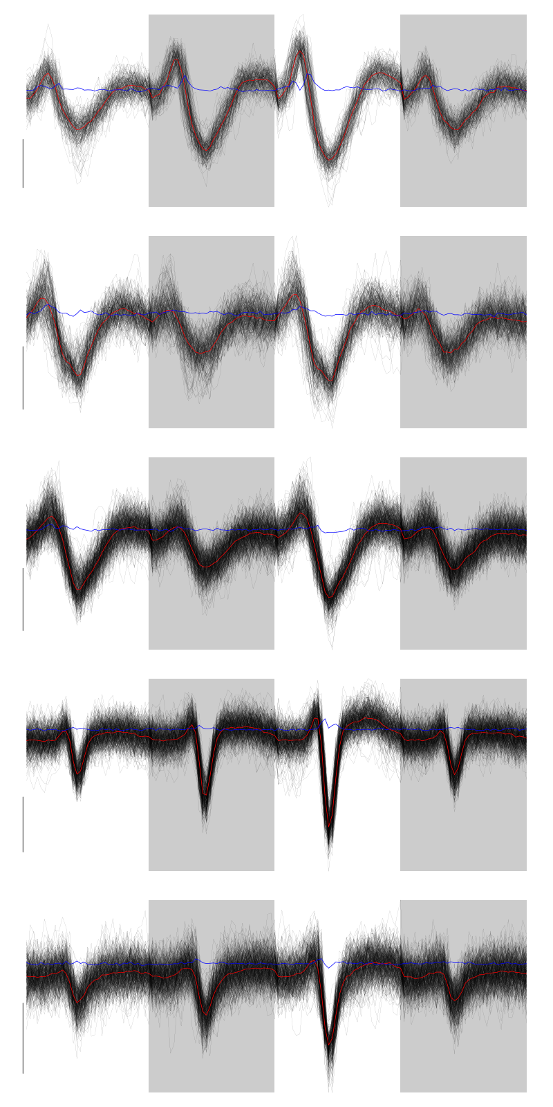
Figure 5: The events of the five clusters of tetrode D2
2 and 3 must be the same, 5 shows evidence on the third site that events were missed (the MAD is going downwards at the valley). We fuse clusters 2 and 3.
nbc=4
labelb[labelb==3]=2
labelb[labelb==4]=3
labelb[labelb==5]=4
We write a new csv file with the data and the labels:
write.csv(cbind(evts.pc$x[,1:4],labelb),file="tetD2b_sorted.csv")
We get a plot showing the events attributed to each unit with:
layout(matrix(1:nbc,nr=nbc))
par(mar=c(1,1,1,1))
for (i in (1:nbc)) {
    ei = labelb==i
    ni = sum(ei)
    plot(evts[,goodEvts][,ei][,1:ifelse(ni>200,200,ni)],y.bar=5)
}
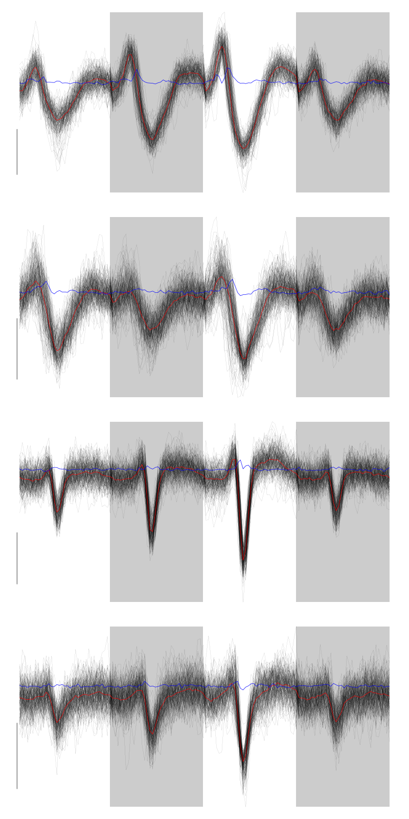
Figure 6: The first 200 events of the four clusters of tetrode D2
2.12 Long cuts creation
For the peeling process we need templates that start and end at 0 (we will otherwise generate artifacts when we subtract). We proceed "as usual" with (I tried first with the default value for parameters before and after but I reduced their values after looking at the centers, see the next figure):
c_before = 49
c_after = 80
centers = lapply(1:nbc, function(i)
    mk_center_list(sp0[goodEvts][labelb==i],lD,
                   before=c_before,after=c_after))
names(centers) = paste("Cluster",1:nbc)
We then make sure that our cuts are long enough by looking at them:
layout(matrix(1:nbc,nr=nbc))
par(mar=c(1,4,1,1))
the_range=c(min(sapply(centers,function(l) min(l$center))),
            max(sapply(centers,function(l) max(l$center))))
for (i in 1:nbc) {
    template = centers[[i]]$center
    plot(template,lwd=2,col=2,
         ylim=the_range,type="l",ylab="")
    abline(h=0,col="grey50")
    abline(v=(1:2)*(c_before+c_after)+1,col="grey50")
    lines(filter(template,rep(1,filter_length)/filter_length),
          col=1,lty=3,lwd=2)
    abline(h=-threshold_factor,col="grey",lty=2,lwd=2)
    lines(centers[[i]]$centerD,lwd=2,col=4)
}
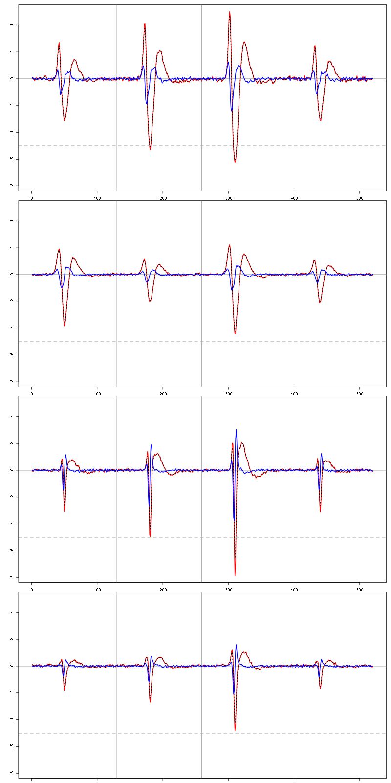
Figure 7: The four templates (red) together with their first derivative (blue) all with the same scale. The dashed black curve show the templates filtered with the filter used during spike detection and the horizontal dashed grey line shows the detection threshold.
Only unit 1 and 3 should reliably pass our threshold…
2.13 Peeling
We can now do the peeling.
2.13.1 Round 0
We classify, predict, subtract and check how many non-classified events we get:
round0 = lapply(as.vector(sp0),classify_and_align_evt,
                data=lD,centers=centers,
                before=c_before,after=c_after)
pred0 = predict_data(round0,centers,data_length = dim(lD)[1])
lD_1 = lD - pred0
sum(sapply(round0, function(l) l[[1]] == '?'))
2
We can see the difference before / after peeling for the data between 1.1 and 1.2 s:
ii = 1:1500 + 1.1*15000
tt = ii/15000
par(mar=c(1,1,1,1))
plot(tt, lD[ii,1], axes = FALSE,
     type="l",ylim=c(-50,10),
     xlab="",ylab="")
lines(tt, lD_1[ii,1], col='red')
lines(tt, lD[ii,2]-15, col='black')
lines(tt, lD_1[ii,2]-15, col='red')
lines(tt, lD[ii,3]-25, col='black')
lines(tt, lD_1[ii,3]-25, col='red')
lines(tt, lD[ii,4]-40, col='black')
lines(tt, lD_1[ii,4]-40, col='red')
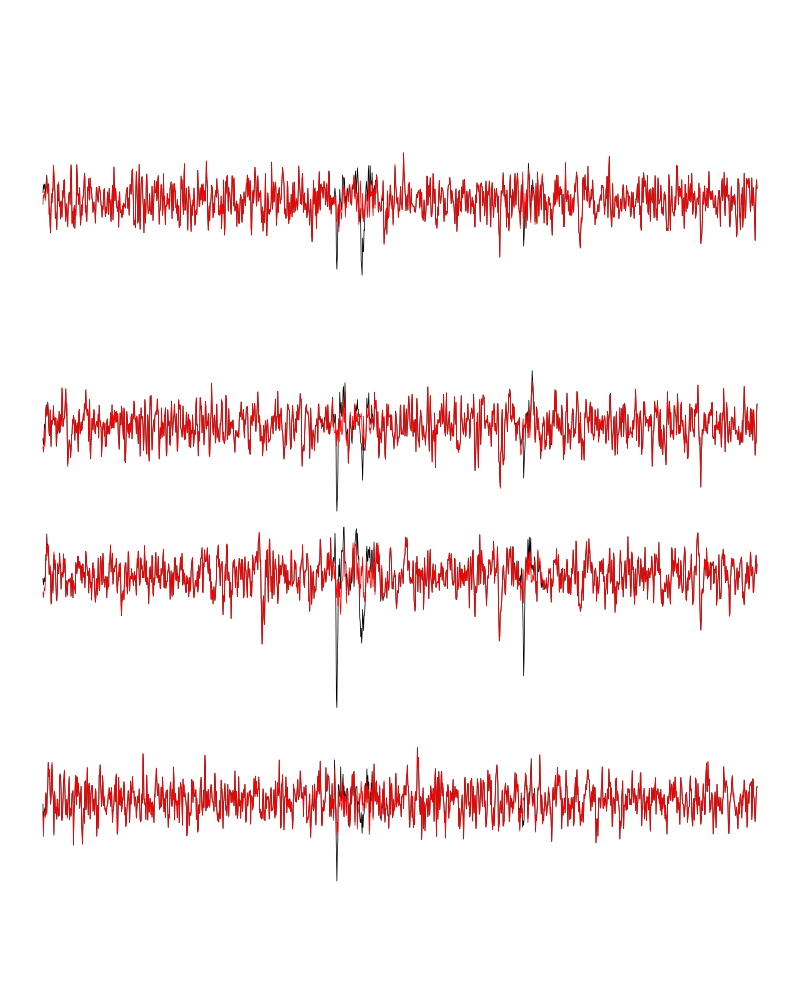
Figure 8: The first peeling illustrated on 100 ms of data, the raw data are in black and the first subtration in red.
2.13.2 Round 1
We keep going, using the subtracted data lD_1 as "raw data", detecting on all sites using the original MAD for normalization and a shorter minimal allowed time between detected spikes:
lDf = -lD_1
lDf = filter(lDf,rep(1,filter_length)/filter_length)
lDf[is.na(lDf)] = 0
lDf = t(t(lDf)/lDf_mad_original)
thrs = threshold_factor*c(1,1,1,1)
bellow.thrs = t(t(lDf) < thrs)
lDfr = lDf
lDfr[bellow.thrs] = 0
remove(lDf)
sp1 = peaks(apply(lDfr,1,sum),10)
remove(lDfr)
sp1
eventsPos object with indexes of 43 events.
  Mean inter event interval: 20903.57 sampling points, corresponding SD: 21759.44 sampling points
  Smallest and largest inter event intervals: 14 and 80499 sampling points.
We classify, predict, subtract and check how many non-classified events we get:
round1 = lapply(as.vector(sp1),classify_and_align_evt,
                data=lD_1,centers=centers,
                before=c_before,after=c_after)
pred1 = predict_data(round1,centers,data_length = dim(lD)[1])
lD_2 = lD_1 - pred1
sum(sapply(round1, function(l) l[[1]] == '?'))
3
We look at what's left with (not shown):
explore(sp1,lD_2,col=c("black","grey50"))
We decide to stop here.
2.14 Getting the spike trains
round_all = c(round0,round1)
spike_trains = lapply(paste("Cluster",1:nbc),
                      function(cn) sort(sapply(round_all[sapply(round_all,
                                                           function(l) l[[1]]==cn)],
                                          function(l) l[[2]]+l[[3]])))
names(spike_trains) = paste("Cluster",1:nbc)
2.15 Getting the inter spike intervals and the forward and backward recurrence times
2.15.1 ISI distributions
We first get the ISI (inter spike intervals) of each unit:
isi = sapply(spike_trains, diff)
names(isi) = names(spike_trains)
We get the ISI ECDF for the four units with:
layout(matrix(1:nbc,nr=nbc/2))
par(mar=c(4,5,6,1))
for (cn in names(isi)) plot_isi(isi[[cn]],main=cn)
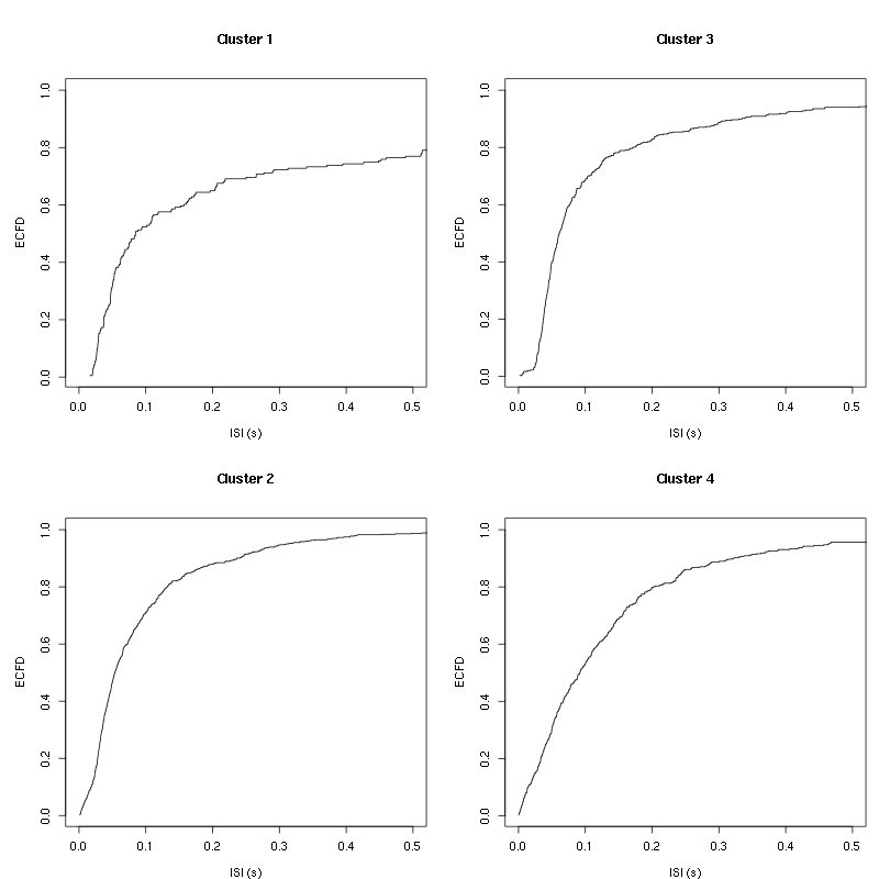
Figure 9: ISI ECDF for the four units.
2.15.2 Forward and Backward Recurrence Times
The forward recurrence time (FRT) between neuron A and B is the elapsed time between a spike in A and the next spike in B. The backward recurrence time (BRT) is the same thing except that we look for the former spike in B. If A and B are not correlated, the expected density of the FRT is the survival function (1-CDF) of the ISI from B divided by the mean ISI of B (the same holds for the BRT under the null hypothesis after taking the opposite). All that is correct if the data are stationary.
On the data at hand that gives:
layout_matrix = matrix(0,nr=nbc,nc=nbc)
counter = 1
for (i in 1:nbc)
    for (j in 1:nbc)
        if (i != j) {
            layout_matrix[i,j] = counter
            counter = counter +1
        }
layout(layout_matrix)
par(mar=c(4,3,4,1))
for (i in 1:nbc)
    for (j in 1:nbc)
        if (i != j)
            test_rt(spike_trains[[i]],
                    spike_trains[[j]],
                    ylab="",main=paste("Units",i,"and",j))
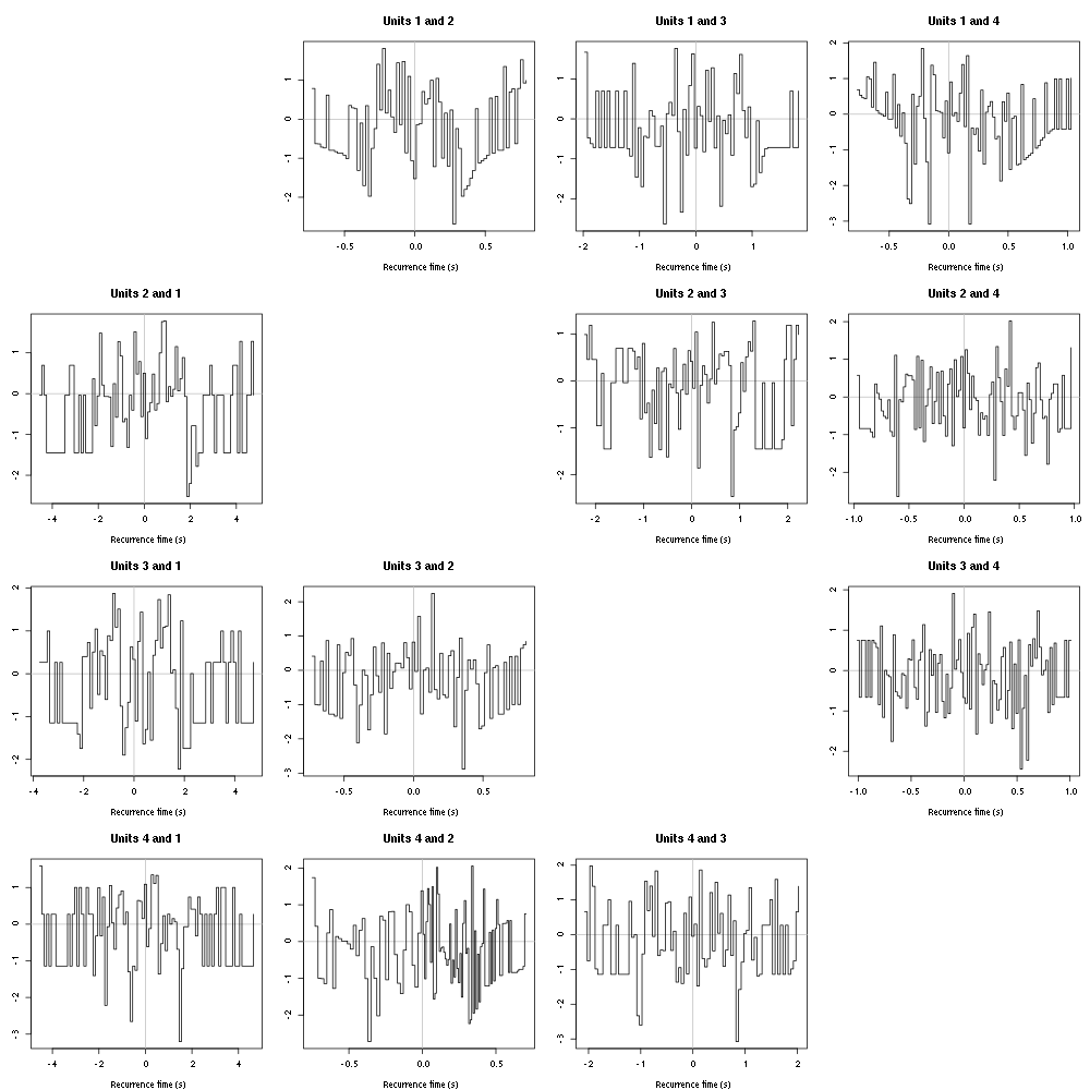
Figure 10: Graphical tests of the Backward and Forward Reccurrence Times distrution agaisnt the null hypothesis (no interaction). If the null is correct, the curves should be IID draws from a standard normal distribution.
2.16 Testing "all at once"
We test the function with:
## We need again an un-normalized version of the data
ref_data = rbind(cbind(h5read("locust20000421.hdf5", "/Spontaneous/ch13"),
                       h5read("locust20000421.hdf5", "/Spontaneous/ch14"),
                       h5read("locust20000421.hdf5", "/Spontaneous/ch15"),
                       h5read("locust20000421.hdf5", "/Spontaneous/ch16")))
## We can now use our function
aao=all_at_once(data=ref_data, centers, thres=threshold_factor*c(1,1,1,1),
                filter_length_1=filter_length, filter_length=filter_length,
                minimalDist_1=15, minimalDist=10,
                before=c_before, after=c_after,
                detection_cycle=c(0,0), verbose=2)
The five number summary is:
       V1             V2             V3             V4
 Min.   :1541   Min.   :1462   Min.   :1267   Min.   :1670
 1st Qu.:2008   1st Qu.:2005   1st Qu.:2022   1st Qu.:2023
 Median :2047   Median :2049   Median :2065   Median :2063
 Mean   :2046   Mean   :2048   Mean   :2063   Mean   :2063
 3rd Qu.:2085   3rd Qu.:2092   3rd Qu.:2106   3rd Qu.:2103
 Max.   :2498   Max.   :2480   Max.   :2612   Max.   :2392

Doing now round 0 detecting on all sites
    Total Cluster 1 Cluster 2 Cluster 3 Cluster 4         ?
     1615       191       609       413       400         2

Doing now round 1 detecting on all sites
    Total Cluster 1 Cluster 2 Cluster 3 Cluster 4         ?
       43         1        16         5        18         3

Global counts at classification's end:
    Total Cluster 1 Cluster 2 Cluster 3 Cluster 4         ?
     1656       192       625       418       418         3
We see that we are getting back the numbers we obtained before step by step.
We can compare the "old" and "new" centers with (not shown):
layout(matrix(1:nbc,nr=nbc))
par(mar=c(1,4,1,1))
for (i in 1:nbc) {
    plot(centers[[i]]$center,lwd=2,col=2,
         ylim=the_range,type="l")
    abline(h=0,col="grey50")
    abline(v=(c_before+c_after)+1,col="grey50")
    lines(aao$centers[[i]]$center,lwd=1,col=4)
}
They are not exactly identical since the new version is computed with all events (superposed or not) attributed to each neuron.
3 Analyzing a sequence of trials
3.1 Create a directory were results get saved
We will carry out an analysis of sequences of 30/25 trials with a given odor. At the end of the analysis of the sequence we will save some intermediate R object in a directory we are now creating.:
if (!dir.exists("tetD2_analysis"))
    dir.create("tetD2_analysis")
3.2 Define a "taylored" version of sort_many_trials
In order to save space and to avoid typos, we define next a taylored version of sort_many_trials:
smt = function(stim_name,
               trial_nbs=1:25,
               centers,
               counts) {
    sort_many_trials(inter_trial_time=10*15000,
                     get_data_fct=function(i,s) get_data(i,s,
                                                         channels = c("ch13","ch14","ch15","ch16"),
                                                         file="locust20000421.hdf5"),
                     stim_name=stim_name,
                     trial_nbs=trial_nbs,
                     centers=centers,
                     counts=counts,
                     all_at_once_call_list=list(thres=threshold_factor*c(1,1,1,1),
                                                filter_length_1=filter_length, filter_length=filter_length,
                                                minimalDist_1=15, minimalDist=10,
                                                before=c_before, after=c_after,
                                                detection_cycle=c(0,0), verbose=1),
                     layout_matrix=matrix(c(1,1:5),nr=3),new_weight_in_update=0.01
                     )
}
4 Systematic analysis of the 30 trials from 1-Hexanol
The LabBook mentions that a drop of solution was added at trial 13 but looking at the data, no major corruption occurs except for a very sharp artifact so we keep that trial.
4.1 Doing the job
a_1_Hexanol_tetD2=smt(stim_name="1-Hexanol",
                      trial_nbs=1:30,
                      centers=aao$centers,
                      counts=aao$counts)
***************
Doing now trial 1 of 1-Hexanol
The five number summary is:
      ch13           ch14           ch15           ch16
 Min.   :1614   Min.   :1478   Min.   :1420   Min.   :1734
 1st Qu.:2007   1st Qu.:2005   1st Qu.:2022   1st Qu.:2022
 Median :2047   Median :2050   Median :2065   Median :2064
 Mean   :2047   Mean   :2049   Mean   :2063   Mean   :2063
 3rd Qu.:2087   3rd Qu.:2094   3rd Qu.:2107   3rd Qu.:2105
 Max.   :2333   Max.   :2436   Max.   :2507   Max.   :2343

Global counts at classification's end:
    Total Cluster 1 Cluster 2 Cluster 3 Cluster 4         ?
      229        16        86        72        55         0
Trial 1 done!
******************
***************
Doing now trial 2 of 1-Hexanol
The five number summary is:
      ch13           ch14           ch15           ch16
 Min.   :1677   Min.   :1469   Min.   :1334   Min.   :1724
 1st Qu.:2007   1st Qu.:2005   1st Qu.:2022   1st Qu.:2022
 Median :2048   Median :2050   Median :2065   Median :2064
 Mean   :2047   Mean   :2049   Mean   :2063   Mean   :2063
 3rd Qu.:2087   3rd Qu.:2094   3rd Qu.:2107   3rd Qu.:2105
 Max.   :2393   Max.   :2522   Max.   :2545   Max.   :2361

Global counts at classification's end:
    Total Cluster 1 Cluster 2 Cluster 3 Cluster 4         ?
      240        17       100        57        66         0
Trial 2 done!
******************
***************
Doing now trial 3 of 1-Hexanol
The five number summary is:
      ch13           ch14           ch15           ch16
 Min.   :1663   Min.   :1495   Min.   :1318   Min.   :1703
 1st Qu.:2007   1st Qu.:2005   1st Qu.:2022   1st Qu.:2022
 Median :2048   Median :2050   Median :2065   Median :2064
 Mean   :2047   Mean   :2049   Mean   :2063   Mean   :2063
 3rd Qu.:2087   3rd Qu.:2094   3rd Qu.:2107   3rd Qu.:2105
 Max.   :2390   Max.   :2444   Max.   :2509   Max.   :2341

Global counts at classification's end:
    Total Cluster 1 Cluster 2 Cluster 3 Cluster 4         ?
      215        20        86        58        51         0
Trial 3 done!
******************
***************
Doing now trial 4 of 1-Hexanol
The five number summary is:
      ch13           ch14           ch15           ch16
 Min.   :1617   Min.   :1407   Min.   :1175   Min.   :1702
 1st Qu.:2008   1st Qu.:2005   1st Qu.:2022   1st Qu.:2022
 Median :2048   Median :2050   Median :2065   Median :2064
 Mean   :2047   Mean   :2049   Mean   :2063   Mean   :2063
 3rd Qu.:2087   3rd Qu.:2093   3rd Qu.:2106   3rd Qu.:2104
 Max.   :2384   Max.   :2514   Max.   :2512   Max.   :2363

Global counts at classification's end:
    Total Cluster 1 Cluster 2 Cluster 3 Cluster 4         ?
      245        12        86        79        68         0
Trial 4 done!
******************
***************
Doing now trial 5 of 1-Hexanol
The five number summary is:
      ch13           ch14           ch15           ch16
 Min.   :1674   Min.   :1567   Min.   :1379   Min.   :1722
 1st Qu.:2007   1st Qu.:2005   1st Qu.:2023   1st Qu.:2022
 Median :2047   Median :2050   Median :2065   Median :2064
 Mean   :2047   Mean   :2049   Mean   :2063   Mean   :2063
 3rd Qu.:2087   3rd Qu.:2093   3rd Qu.:2106   3rd Qu.:2105
 Max.   :2393   Max.   :2457   Max.   :2466   Max.   :2360

Global counts at classification's end:
    Total Cluster 1 Cluster 2 Cluster 3 Cluster 4         ?
      210        10       105        34        60         1
Trial 5 done!
******************
***************
Doing now trial 6 of 1-Hexanol
The five number summary is:
      ch13           ch14           ch15           ch16
 Min.   :1645   Min.   :1554   Min.   :1366   Min.   :1709
 1st Qu.:2007   1st Qu.:2005   1st Qu.:2022   1st Qu.:2022
 Median :2048   Median :2050   Median :2065   Median :2064
 Mean   :2047   Mean   :2049   Mean   :2063   Mean   :2063
 3rd Qu.:2087   3rd Qu.:2094   3rd Qu.:2107   3rd Qu.:2105
 Max.   :2360   Max.   :2459   Max.   :2494   Max.   :2365

Global counts at classification's end:
    Total Cluster 1 Cluster 2 Cluster 3 Cluster 4         ?
      219        20        81        66        52         0
Trial 6 done!
******************
***************
Doing now trial 7 of 1-Hexanol
The five number summary is:
      ch13           ch14           ch15           ch16
 Min.   :1660   Min.   :1500   Min.   :1421   Min.   :1729
 1st Qu.:2007   1st Qu.:2005   1st Qu.:2022   1st Qu.:2022
 Median :2048   Median :2050   Median :2065   Median :2064
 Mean   :2047   Mean   :2049   Mean   :2063   Mean   :2063
 3rd Qu.:2087   3rd Qu.:2094   3rd Qu.:2107   3rd Qu.:2105
 Max.   :2361   Max.   :2505   Max.   :2519   Max.   :2381

Global counts at classification's end:
    Total Cluster 1 Cluster 2 Cluster 3 Cluster 4         ?
      213        21        92        46        54         0
Trial 7 done!
******************
***************
Doing now trial 8 of 1-Hexanol
The five number summary is:
      ch13           ch14           ch15           ch16
 Min.   :1638   Min.   :1511   Min.   :1276   Min.   :1727
 1st Qu.:2007   1st Qu.:2005   1st Qu.:2022   1st Qu.:2022
 Median :2048   Median :2051   Median :2065   Median :2064
 Mean   :2047   Mean   :2049   Mean   :2063   Mean   :2063
 3rd Qu.:2088   3rd Qu.:2094   3rd Qu.:2107   3rd Qu.:2105
 Max.   :2373   Max.   :2450   Max.   :2494   Max.   :2349

Global counts at classification's end:
    Total Cluster 1 Cluster 2 Cluster 3 Cluster 4         ?
      243        32        86        71        54         0
Trial 8 done!
******************
***************
Doing now trial 9 of 1-Hexanol
The five number summary is:
      ch13           ch14           ch15           ch16
 Min.   :1674   Min.   :1510   Min.   :1356   Min.   :1715
 1st Qu.:2007   1st Qu.:2005   1st Qu.:2022   1st Qu.:2022
 Median :2047   Median :2051   Median :2065   Median :2064
 Mean   :2047   Mean   :2049   Mean   :2063   Mean   :2063
 3rd Qu.:2088   3rd Qu.:2094   3rd Qu.:2107   3rd Qu.:2105
 Max.   :2363   Max.   :2438   Max.   :2499   Max.   :2381

Global counts at classification's end:
    Total Cluster 1 Cluster 2 Cluster 3 Cluster 4         ?
      239        16        97        74        52         0
Trial 9 done!
******************
***************
Doing now trial 10 of 1-Hexanol
The five number summary is:
      ch13           ch14           ch15           ch16
 Min.   :1613   Min.   :1491   Min.   :1402   Min.   :1668
 1st Qu.:2007   1st Qu.:2004   1st Qu.:2022   1st Qu.:2022
 Median :2048   Median :2050   Median :2065   Median :2064
 Mean   :2047   Mean   :2049   Mean   :2063   Mean   :2063
 3rd Qu.:2088   3rd Qu.:2095   3rd Qu.:2108   3rd Qu.:2105
 Max.   :2364   Max.   :2531   Max.   :2521   Max.   :2325

Global counts at classification's end:
    Total Cluster 1 Cluster 2 Cluster 3 Cluster 4         ?
      240        26        74        79        60         1
Trial 10 done!
******************
***************
Doing now trial 11 of 1-Hexanol
The five number summary is:
      ch13           ch14           ch15           ch16
 Min.   :1622   Min.   :1398   Min.   :1328   Min.   :1577
 1st Qu.:2007   1st Qu.:2005   1st Qu.:2022   1st Qu.:2022
 Median :2048   Median :2050   Median :2065   Median :2064
 Mean   :2047   Mean   :2049   Mean   :2063   Mean   :2063
 3rd Qu.:2088   3rd Qu.:2094   3rd Qu.:2107   3rd Qu.:2105
 Max.   :2369   Max.   :2520   Max.   :2603   Max.   :2341

Global counts at classification's end:
    Total Cluster 1 Cluster 2 Cluster 3 Cluster 4         ?
      246        38        73        57        77         1
Trial 11 done!
******************
***************
Doing now trial 12 of 1-Hexanol
The five number summary is:
      ch13           ch14           ch15           ch16
 Min.   :1698   Min.   :1495   Min.   :1425   Min.   :1755
 1st Qu.:2007   1st Qu.:2005   1st Qu.:2022   1st Qu.:2022
 Median :2047   Median :2050   Median :2065   Median :2064
 Mean   :2047   Mean   :2049   Mean   :2063   Mean   :2063
 3rd Qu.:2088   3rd Qu.:2094   3rd Qu.:2107   3rd Qu.:2105
 Max.   :2374   Max.   :2476   Max.   :2489   Max.   :2389

Global counts at classification's end:
    Total Cluster 1 Cluster 2 Cluster 3 Cluster 4         ?
      201        17        71        48        65         0
Trial 12 done!
******************
***************
Doing now trial 13 of 1-Hexanol
The five number summary is:
      ch13           ch14           ch15           ch16
 Min.   :1528   Min.   :1430   Min.   :1275   Min.   :1314
 1st Qu.:2007   1st Qu.:2005   1st Qu.:2022   1st Qu.:2022
 Median :2048   Median :2051   Median :2066   Median :2065
 Mean   :2047   Mean   :2049   Mean   :2063   Mean   :2063
 3rd Qu.:2088   3rd Qu.:2094   3rd Qu.:2107   3rd Qu.:2105
 Max.   :4095   Max.   :4095   Max.   :4095   Max.   :4095

Global counts at classification's end:
    Total Cluster 1 Cluster 2 Cluster 3 Cluster 4         ?
      213         5        71        61        74         2
Trial 13 done!
******************
***************
Doing now trial 14 of 1-Hexanol
The five number summary is:
      ch13           ch14           ch15           ch16
 Min.   :1607   Min.   :1468   Min.   :1304   Min.   :1696
 1st Qu.:2007   1st Qu.:2005   1st Qu.:2022   1st Qu.:2022
 Median :2048   Median :2050   Median :2065   Median :2064
 Mean   :2047   Mean   :2049   Mean   :2063   Mean   :2063
 3rd Qu.:2088   3rd Qu.:2095   3rd Qu.:2107   3rd Qu.:2105
 Max.   :2375   Max.   :2522   Max.   :2528   Max.   :2401

Global counts at classification's end:
    Total Cluster 1 Cluster 2 Cluster 3 Cluster 4         ?
      226        42        62        65        55         2
Trial 14 done!
******************
***************
Doing now trial 15 of 1-Hexanol
The five number summary is:
      ch13           ch14           ch15           ch16
 Min.   :1693   Min.   :1490   Min.   :1385   Min.   :1727
 1st Qu.:2007   1st Qu.:2005   1st Qu.:2022   1st Qu.:2022
 Median :2048   Median :2050   Median :2065   Median :2064
 Mean   :2047   Mean   :2049   Mean   :2063   Mean   :2063
 3rd Qu.:2087   3rd Qu.:2094   3rd Qu.:2107   3rd Qu.:2105
 Max.   :2378   Max.   :2524   Max.   :2536   Max.   :2351

Global counts at classification's end:
    Total Cluster 1 Cluster 2 Cluster 3 Cluster 4         ?
      192        18        57        60        57         0
Trial 15 done!
******************
***************
Doing now trial 16 of 1-Hexanol
The five number summary is:
      ch13           ch14           ch15           ch16
 Min.   :1567   Min.   :1469   Min.   :1279   Min.   :1689
 1st Qu.:2008   1st Qu.:2005   1st Qu.:2022   1st Qu.:2022
 Median :2048   Median :2051   Median :2065   Median :2065
 Mean   :2047   Mean   :2049   Mean   :2063   Mean   :2063
 3rd Qu.:2088   3rd Qu.:2094   3rd Qu.:2107   3rd Qu.:2105
 Max.   :2349   Max.   :2458   Max.   :2499   Max.   :2386

Global counts at classification's end:
    Total Cluster 1 Cluster 2 Cluster 3 Cluster 4         ?
      211        18        79        63        50         1
Trial 16 done!
******************
***************
Doing now trial 17 of 1-Hexanol
The five number summary is:
      ch13           ch14           ch15           ch16
 Min.   :1681   Min.   :1523   Min.   :1267   Min.   :1706
 1st Qu.:2007   1st Qu.:2005   1st Qu.:2022   1st Qu.:2022
 Median :2048   Median :2050   Median :2065   Median :2064
 Mean   :2047   Mean   :2049   Mean   :2063   Mean   :2063
 3rd Qu.:2087   3rd Qu.:2094   3rd Qu.:2107   3rd Qu.:2105
 Max.   :2333   Max.   :2465   Max.   :2513   Max.   :2343

Global counts at classification's end:
    Total Cluster 1 Cluster 2 Cluster 3 Cluster 4         ?
      196        17        67        58        54         0
Trial 17 done!
******************
***************
Doing now trial 18 of 1-Hexanol
The five number summary is:
      ch13           ch14           ch15           ch16
 Min.   :1656   Min.   :1413   Min.   :1312   Min.   :1675
 1st Qu.:2007   1st Qu.:2005   1st Qu.:2022   1st Qu.:2022
 Median :2048   Median :2051   Median :2065   Median :2064
 Mean   :2047   Mean   :2049   Mean   :2063   Mean   :2063
 3rd Qu.:2088   3rd Qu.:2095   3rd Qu.:2107   3rd Qu.:2105
 Max.   :2358   Max.   :2458   Max.   :2513   Max.   :2343

Global counts at classification's end:
    Total Cluster 1 Cluster 2 Cluster 3 Cluster 4         ?
      216        32        64        80        40         0
Trial 18 done!
******************
***************
Doing now trial 19 of 1-Hexanol
The five number summary is:
      ch13           ch14           ch15           ch16
 Min.   :1664   Min.   :1475   Min.   :1360   Min.   :1745
 1st Qu.:2007   1st Qu.:2005   1st Qu.:2022   1st Qu.:2022
 Median :2048   Median :2050   Median :2066   Median :2064
 Mean   :2047   Mean   :2049   Mean   :2063   Mean   :2063
 3rd Qu.:2088   3rd Qu.:2095   3rd Qu.:2108   3rd Qu.:2106
 Max.   :2397   Max.   :2496   Max.   :2559   Max.   :2380

Global counts at classification's end:
    Total Cluster 1 Cluster 2 Cluster 3 Cluster 4         ?
      259        21        76        97        64         1
Trial 19 done!
******************
***************
Doing now trial 20 of 1-Hexanol
The five number summary is:
      ch13           ch14           ch15           ch16
 Min.   :1604   Min.   :1479   Min.   :1444   Min.   :1729
 1st Qu.:2008   1st Qu.:2005   1st Qu.:2022   1st Qu.:2022
 Median :2048   Median :2051   Median :2065   Median :2064
 Mean   :2047   Mean   :2049   Mean   :2063   Mean   :2063
 3rd Qu.:2088   3rd Qu.:2094   3rd Qu.:2107   3rd Qu.:2105
 Max.   :2352   Max.   :2503   Max.   :2557   Max.   :2365

Global counts at classification's end:
    Total Cluster 1 Cluster 2 Cluster 3 Cluster 4         ?
      203        16        72        50        65         0
Trial 20 done!
******************
***************
Doing now trial 21 of 1-Hexanol
The five number summary is:
      ch13           ch14           ch15           ch16
 Min.   :1667   Min.   :1516   Min.   :1385   Min.   :1683
 1st Qu.:2007   1st Qu.:2005   1st Qu.:2022   1st Qu.:2022
 Median :2048   Median :2051   Median :2066   Median :2064
 Mean   :2047   Mean   :2049   Mean   :2063   Mean   :2063
 3rd Qu.:2088   3rd Qu.:2094   3rd Qu.:2107   3rd Qu.:2105
 Max.   :2343   Max.   :2437   Max.   :2614   Max.   :2481

Global counts at classification's end:
    Total Cluster 1 Cluster 2 Cluster 3 Cluster 4         ?
      244        14        90        71        69         0
Trial 21 done!
******************
***************
Doing now trial 22 of 1-Hexanol
The five number summary is:
      ch13           ch14           ch15           ch16
 Min.   :1693   Min.   :1446   Min.   :1370   Min.   :1681
 1st Qu.:2007   1st Qu.:2005   1st Qu.:2022   1st Qu.:2022
 Median :2048   Median :2051   Median :2066   Median :2065
 Mean   :2047   Mean   :2049   Mean   :2063   Mean   :2063
 3rd Qu.:2088   3rd Qu.:2094   3rd Qu.:2107   3rd Qu.:2105
 Max.   :2357   Max.   :2531   Max.   :2512   Max.   :2387

Global counts at classification's end:
    Total Cluster 1 Cluster 2 Cluster 3 Cluster 4         ?
      221        38        65        57        61         0
Trial 22 done!
******************
***************
Doing now trial 23 of 1-Hexanol
The five number summary is:
      ch13           ch14           ch15           ch16
 Min.   :1658   Min.   :1479   Min.   :1367   Min.   :1641
 1st Qu.:2008   1st Qu.:2005   1st Qu.:2022   1st Qu.:2022
 Median :2048   Median :2051   Median :2065   Median :2065
 Mean   :2047   Mean   :2049   Mean   :2063   Mean   :2063
 3rd Qu.:2088   3rd Qu.:2094   3rd Qu.:2107   3rd Qu.:2105
 Max.   :2352   Max.   :2514   Max.   :2549   Max.   :2382

Global counts at classification's end:
    Total Cluster 1 Cluster 2 Cluster 3 Cluster 4         ?
      214        23        73        71        46         1
Trial 23 done!
******************
***************
Doing now trial 24 of 1-Hexanol
The five number summary is:
      ch13           ch14           ch15           ch16
 Min.   :1597   Min.   :1424   Min.   :1387   Min.   :1732
 1st Qu.:2008   1st Qu.:2005   1st Qu.:2022   1st Qu.:2023
 Median :2048   Median :2051   Median :2066   Median :2064
 Mean   :2047   Mean   :2049   Mean   :2063   Mean   :2063
 3rd Qu.:2088   3rd Qu.:2094   3rd Qu.:2107   3rd Qu.:2105
 Max.   :2377   Max.   :2455   Max.   :2526   Max.   :2355

Global counts at classification's end:
    Total Cluster 1 Cluster 2 Cluster 3 Cluster 4         ?
      254        32        90        76        55         1
Trial 24 done!
******************
***************
Doing now trial 25 of 1-Hexanol
The five number summary is:
      ch13           ch14           ch15           ch16
 Min.   :1559   Min.   :1523   Min.   :1399   Min.   :1728
 1st Qu.:2008   1st Qu.:2005   1st Qu.:2023   1st Qu.:2022
 Median :2048   Median :2051   Median :2065   Median :2065
 Mean   :2047   Mean   :2049   Mean   :2063   Mean   :2063
 3rd Qu.:2087   3rd Qu.:2094   3rd Qu.:2107   3rd Qu.:2105
 Max.   :2335   Max.   :2433   Max.   :2500   Max.   :2375

Global counts at classification's end:
    Total Cluster 1 Cluster 2 Cluster 3 Cluster 4         ?
      240        29        79        58        73         1
Trial 25 done!
******************
***************
Doing now trial 26 of 1-Hexanol
The five number summary is:
      ch13           ch14           ch15           ch16
 Min.   :1680   Min.   :1411   Min.   :1322   Min.   :1736
 1st Qu.:2008   1st Qu.:2006   1st Qu.:2023   1st Qu.:2023
 Median :2048   Median :2051   Median :2065   Median :2065
 Mean   :2047   Mean   :2049   Mean   :2063   Mean   :2063
 3rd Qu.:2087   3rd Qu.:2094   3rd Qu.:2107   3rd Qu.:2104
 Max.   :2371   Max.   :2493   Max.   :2484   Max.   :2325

Global counts at classification's end:
    Total Cluster 1 Cluster 2 Cluster 3 Cluster 4         ?
      221        22        67        75        57         0
Trial 26 done!
******************
***************
Doing now trial 27 of 1-Hexanol
The five number summary is:
      ch13           ch14           ch15           ch16
 Min.   :1669   Min.   :1458   Min.   :1403   Min.   :1681
 1st Qu.:2008   1st Qu.:2006   1st Qu.:2023   1st Qu.:2022
 Median :2048   Median :2051   Median :2065   Median :2065
 Mean   :2047   Mean   :2049   Mean   :2063   Mean   :2063
 3rd Qu.:2087   3rd Qu.:2095   3rd Qu.:2107   3rd Qu.:2105
 Max.   :2386   Max.   :2484   Max.   :2460   Max.   :2381

Global counts at classification's end:
    Total Cluster 1 Cluster 2 Cluster 3 Cluster 4         ?
      262        45        73        75        69         0
Trial 27 done!
******************
***************
Doing now trial 28 of 1-Hexanol
The five number summary is:
      ch13           ch14           ch15           ch16
 Min.   :1643   Min.   :1413   Min.   :1244   Min.   :1719
 1st Qu.:2008   1st Qu.:2006   1st Qu.:2023   1st Qu.:2023
 Median :2048   Median :2050   Median :2065   Median :2065
 Mean   :2047   Mean   :2049   Mean   :2063   Mean   :2063
 3rd Qu.:2087   3rd Qu.:2094   3rd Qu.:2106   3rd Qu.:2104
 Max.   :2330   Max.   :2527   Max.   :2450   Max.   :2345

Global counts at classification's end:
    Total Cluster 1 Cluster 2 Cluster 3 Cluster 4         ?
      207        12        66        72        57         0
Trial 28 done!
******************
***************
Doing now trial 29 of 1-Hexanol
The five number summary is:
      ch13           ch14           ch15           ch16
 Min.   :1653   Min.   :1542   Min.   :1395   Min.   :1710
 1st Qu.:2008   1st Qu.:2006   1st Qu.:2023   1st Qu.:2023
 Median :2048   Median :2051   Median :2066   Median :2064
 Mean   :2047   Mean   :2049   Mean   :2063   Mean   :2063
 3rd Qu.:2087   3rd Qu.:2093   3rd Qu.:2106   3rd Qu.:2104
 Max.   :2308   Max.   :2474   Max.   :2563   Max.   :2388

Global counts at classification's end:
    Total Cluster 1 Cluster 2 Cluster 3 Cluster 4         ?
      212        12        79        53        68         0
Trial 29 done!
******************
***************
Doing now trial 30 of 1-Hexanol
The five number summary is:
      ch13           ch14           ch15           ch16
 Min.   :1645   Min.   :1488   Min.   :1385   Min.   :1718
 1st Qu.:2009   1st Qu.:2007   1st Qu.:2024   1st Qu.:2024
 Median :2048   Median :2051   Median :2065   Median :2064
 Mean   :2047   Mean   :2049   Mean   :2063   Mean   :2063
 3rd Qu.:2086   3rd Qu.:2093   3rd Qu.:2105   3rd Qu.:2103
 Max.   :2343   Max.   :2407   Max.   :2484   Max.   :2378

Global counts at classification's end:
    Total Cluster 1 Cluster 2 Cluster 3 Cluster 4         ?
      209         2        69        64        72         2
Trial 30 done!
******************
4.2 Diagnostic plots
The counts evolution is:
counts_evolution(a_1_Hexanol_tetD2)

Figure 11: Evolution of the number of events attributed to each unit (1 to 4) or unclassified ("?") during the 30 trials of 1-Hexanol for tetrode D2.
The waveform evolution is:
waveform_evolution(a_1_Hexanol_tetD2,threshold_factor)

Figure 12: Evolution of the templates of each unit during the 30 trials with 1-Hexanol for tetrode D2.
The observed counting processes, inter spike intervals densities ad raster plots are:
cp_isi_raster(a_1_Hexanol_tetD2)
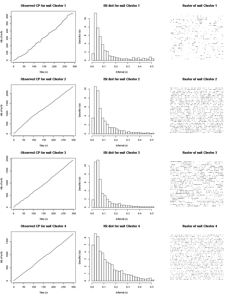
Figure 13: Observed counting processes, empirical inter spike interval distributions and raster plots for 1-Hexanol.
4.3 Save results
Before analyzing the next set of trials we save the output of smt to disk with:
save(a_1_Hexanol_tetD2,
     file=paste0("tetD2_analysis/tetD2_","1-Hexanol","_summary_obj.rda"))
We write to disk the spike trains in text mode:
for (c_idx in 1:length(a_1_Hexanol_tetD2$spike_trains))
    cat(a_1_Hexanol_tetD2$spike_trains[[c_idx]],
        file=paste0("locust20000421_spike_trains/locust20000421_1-Hexanol_tetD2_u",c_idx,".txt"),sep="\n")
5 25 trials with Hexanal
We will carry out an analysis of the 25 trials from Hexanal. The LabBook mentions that a drop of solution was added at trial 18 but looking at the data, no major corruption occurs except for a very sharp artifact:
5.1 Do the job
a_Hexanal_tetD2=smt(stim_name="Hexanal",
                    centers=a_1_Hexanol_tetD2$centers,
                    counts=a_1_Hexanol_tetD2$counts)
***************
Doing now trial 1 of Hexanal
The five number summary is:
      ch13           ch14           ch15           ch16
 Min.   :1636   Min.   :1456   Min.   :1395   Min.   :1744
 1st Qu.:2009   1st Qu.:2007   1st Qu.:2024   1st Qu.:2024
 Median :2048   Median :2051   Median :2066   Median :2065
 Mean   :2047   Mean   :2050   Mean   :2064   Mean   :2064
 3rd Qu.:2086   3rd Qu.:2094   3rd Qu.:2106   3rd Qu.:2104
 Max.   :2383   Max.   :2430   Max.   :2465   Max.   :2344

Global counts at classification's end:
    Total Cluster 1 Cluster 2 Cluster 3 Cluster 4         ?
      257        27        64        80        86         0
Trial 1 done!
******************
***************
Doing now trial 2 of Hexanal
The five number summary is:
      ch13           ch14           ch15           ch16
 Min.   :1650   Min.   :1459   Min.   :1380   Min.   :1694
 1st Qu.:2009   1st Qu.:2007   1st Qu.:2024   1st Qu.:2024
 Median :2049   Median :2051   Median :2066   Median :2065
 Mean   :2047   Mean   :2050   Mean   :2064   Mean   :2064
 3rd Qu.:2087   3rd Qu.:2094   3rd Qu.:2106   3rd Qu.:2104
 Max.   :2377   Max.   :2433   Max.   :2504   Max.   :2341

Global counts at classification's end:
    Total Cluster 1 Cluster 2 Cluster 3 Cluster 4         ?
      252        16        80        87        69         0
Trial 2 done!
******************
***************
Doing now trial 3 of Hexanal
The five number summary is:
      ch13           ch14           ch15           ch16
 Min.   :1644   Min.   :1481   Min.   :1393   Min.   :1700
 1st Qu.:2009   1st Qu.:2007   1st Qu.:2024   1st Qu.:2024
 Median :2048   Median :2051   Median :2066   Median :2065
 Mean   :2047   Mean   :2050   Mean   :2064   Mean   :2064
 3rd Qu.:2086   3rd Qu.:2094   3rd Qu.:2106   3rd Qu.:2104
 Max.   :2362   Max.   :2407   Max.   :2439   Max.   :2330

Global counts at classification's end:
    Total Cluster 1 Cluster 2 Cluster 3 Cluster 4         ?
      260        12        67        96        85         0
Trial 3 done!
******************
***************
Doing now trial 4 of Hexanal
The five number summary is:
      ch13           ch14           ch15           ch16
 Min.   :1627   Min.   :1429   Min.   :1185   Min.   :1698
 1st Qu.:2009   1st Qu.:2007   1st Qu.:2024   1st Qu.:2024
 Median :2049   Median :2051   Median :2066   Median :2065
 Mean   :2047   Mean   :2050   Mean   :2064   Mean   :2064
 3rd Qu.:2087   3rd Qu.:2094   3rd Qu.:2106   3rd Qu.:2104
 Max.   :2327   Max.   :2417   Max.   :2556   Max.   :2329

Global counts at classification's end:
    Total Cluster 1 Cluster 2 Cluster 3 Cluster 4         ?
      284        12       104       103        65         0
Trial 4 done!
******************
***************
Doing now trial 5 of Hexanal
The five number summary is:
      ch13           ch14           ch15           ch16
 Min.   :1629   Min.   :1513   Min.   :1422   Min.   :1723
 1st Qu.:2009   1st Qu.:2007   1st Qu.:2024   1st Qu.:2024
 Median :2048   Median :2051   Median :2066   Median :2065
 Mean   :2047   Mean   :2050   Mean   :2064   Mean   :2064
 3rd Qu.:2086   3rd Qu.:2093   3rd Qu.:2105   3rd Qu.:2104
 Max.   :2318   Max.   :2425   Max.   :2428   Max.   :2345

Global counts at classification's end:
    Total Cluster 1 Cluster 2 Cluster 3 Cluster 4         ?
      208        15        63        57        73         0
Trial 5 done!
******************
***************
Doing now trial 6 of Hexanal
The five number summary is:
      ch13           ch14           ch15           ch16
 Min.   :1671   Min.   :1447   Min.   :1402   Min.   :1733
 1st Qu.:2009   1st Qu.:2007   1st Qu.:2025   1st Qu.:2024
 Median :2048   Median :2051   Median :2066   Median :2065
 Mean   :2047   Mean   :2050   Mean   :2064   Mean   :2064
 3rd Qu.:2086   3rd Qu.:2094   3rd Qu.:2105   3rd Qu.:2104
 Max.   :2332   Max.   :2530   Max.   :2490   Max.   :2372

Global counts at classification's end:
    Total Cluster 1 Cluster 2 Cluster 3 Cluster 4         ?
      205        27        40        56        80         2
Trial 6 done!
******************
***************
Doing now trial 7 of Hexanal
The five number summary is:
      ch13           ch14           ch15           ch16
 Min.   :1638   Min.   :1516   Min.   :1466   Min.   :1730
 1st Qu.:2010   1st Qu.:2007   1st Qu.:2024   1st Qu.:2024
 Median :2048   Median :2051   Median :2066   Median :2065
 Mean   :2047   Mean   :2050   Mean   :2064   Mean   :2064
 3rd Qu.:2086   3rd Qu.:2093   3rd Qu.:2106   3rd Qu.:2104
 Max.   :2368   Max.   :2432   Max.   :2459   Max.   :2337

Global counts at classification's end:
    Total Cluster 1 Cluster 2 Cluster 3 Cluster 4         ?
      240        11        66        69        94         0
Trial 7 done!
******************
***************
Doing now trial 8 of Hexanal
The five number summary is:
      ch13           ch14           ch15           ch16
 Min.   :1601   Min.   :1460   Min.   :1393   Min.   :1705
 1st Qu.:2010   1st Qu.:2008   1st Qu.:2024   1st Qu.:2024
 Median :2048   Median :2051   Median :2066   Median :2065
 Mean   :2047   Mean   :2050   Mean   :2064   Mean   :2064
 3rd Qu.:2086   3rd Qu.:2093   3rd Qu.:2105   3rd Qu.:2104
 Max.   :2326   Max.   :2454   Max.   :2535   Max.   :2356

Global counts at classification's end:
    Total Cluster 1 Cluster 2 Cluster 3 Cluster 4         ?
      219        15        62        75        66         1
Trial 8 done!
******************
***************
Doing now trial 9 of Hexanal
The five number summary is:
      ch13           ch14           ch15           ch16
 Min.   :1657   Min.   :1456   Min.   :1278   Min.   :1673
 1st Qu.:2010   1st Qu.:2007   1st Qu.:2024   1st Qu.:2025
 Median :2048   Median :2051   Median :2066   Median :2065
 Mean   :2047   Mean   :2050   Mean   :2064   Mean   :2064
 3rd Qu.:2086   3rd Qu.:2093   3rd Qu.:2106   3rd Qu.:2103
 Max.   :2393   Max.   :2446   Max.   :2457   Max.   :2346

Global counts at classification's end:
    Total Cluster 1 Cluster 2 Cluster 3 Cluster 4         ?
      252        11        79        93        69         0
Trial 9 done!
******************
***************
Doing now trial 10 of Hexanal
The five number summary is:
      ch13           ch14           ch15           ch16
 Min.   :1646   Min.   :1458   Min.   :1318   Min.   :1714
 1st Qu.:2010   1st Qu.:2007   1st Qu.:2025   1st Qu.:2025
 Median :2048   Median :2051   Median :2066   Median :2065
 Mean   :2047   Mean   :2050   Mean   :2064   Mean   :2064
 3rd Qu.:2086   3rd Qu.:2093   3rd Qu.:2105   3rd Qu.:2103
 Max.   :2353   Max.   :2410   Max.   :2445   Max.   :2355

Global counts at classification's end:
    Total Cluster 1 Cluster 2 Cluster 3 Cluster 4         ?
      247        17        73        72        85         0
Trial 10 done!
******************
***************
Doing now trial 11 of Hexanal
The five number summary is:
      ch13           ch14           ch15           ch16
 Min.   :1644   Min.   :1451   Min.   :1290   Min.   :1698
 1st Qu.:2010   1st Qu.:2008   1st Qu.:2025   1st Qu.:2025
 Median :2048   Median :2051   Median :2066   Median :2065
 Mean   :2047   Mean   :2050   Mean   :2064   Mean   :2064
 3rd Qu.:2086   3rd Qu.:2093   3rd Qu.:2105   3rd Qu.:2103
 Max.   :2397   Max.   :2446   Max.   :2451   Max.   :2333

Global counts at classification's end:
    Total Cluster 1 Cluster 2 Cluster 3 Cluster 4         ?
      218        18        46        86        68         0
Trial 11 done!
******************
***************
Doing now trial 12 of Hexanal
The five number summary is:
      ch13           ch14           ch15           ch16
 Min.   :1637   Min.   :1512   Min.   :1382   Min.   :1729
 1st Qu.:2010   1st Qu.:2008   1st Qu.:2025   1st Qu.:2025
 Median :2049   Median :2051   Median :2066   Median :2065
 Mean   :2047   Mean   :2050   Mean   :2064   Mean   :2064
 3rd Qu.:2086   3rd Qu.:2093   3rd Qu.:2105   3rd Qu.:2103
 Max.   :2337   Max.   :2423   Max.   :2533   Max.   :2314

Global counts at classification's end:
    Total Cluster 1 Cluster 2 Cluster 3 Cluster 4         ?
      233        24        62        59        85         3
Trial 12 done!
******************
***************
Doing now trial 13 of Hexanal
The five number summary is:
      ch13           ch14           ch15           ch16
 Min.   :1607   Min.   :1511   Min.   :1409   Min.   :1710
 1st Qu.:2010   1st Qu.:2008   1st Qu.:2025   1st Qu.:2025
 Median :2049   Median :2051   Median :2066   Median :2065
 Mean   :2048   Mean   :2050   Mean   :2064   Mean   :2064
 3rd Qu.:2086   3rd Qu.:2093   3rd Qu.:2106   3rd Qu.:2104
 Max.   :2327   Max.   :2421   Max.   :2400   Max.   :2359

Global counts at classification's end:
    Total Cluster 1 Cluster 2 Cluster 3 Cluster 4         ?
      274        20        76        91        87         0
Trial 13 done!
******************
***************
Doing now trial 14 of Hexanal
The five number summary is:
      ch13           ch14           ch15           ch16
 Min.   :1640   Min.   :1483   Min.   :1443   Min.   :1697
 1st Qu.:2010   1st Qu.:2007   1st Qu.:2025   1st Qu.:2025
 Median :2049   Median :2051   Median :2066   Median :2065
 Mean   :2048   Mean   :2050   Mean   :2064   Mean   :2064
 3rd Qu.:2086   3rd Qu.:2094   3rd Qu.:2106   3rd Qu.:2104
 Max.   :2421   Max.   :2444   Max.   :2479   Max.   :2350

Global counts at classification's end:
    Total Cluster 1 Cluster 2 Cluster 3 Cluster 4         ?
      278        18        85        63       111         1
Trial 14 done!
******************
***************
Doing now trial 15 of Hexanal
The five number summary is:
      ch13           ch14           ch15           ch16
 Min.   :1634   Min.   :1452   Min.   :1371   Min.   :1716
 1st Qu.:2010   1st Qu.:2008   1st Qu.:2025   1st Qu.:2025
 Median :2049   Median :2051   Median :2066   Median :2065
 Mean   :2048   Mean   :2050   Mean   :2064   Mean   :2064
 3rd Qu.:2086   3rd Qu.:2093   3rd Qu.:2105   3rd Qu.:2103
 Max.   :2331   Max.   :2423   Max.   :2452   Max.   :2327

Global counts at classification's end:
    Total Cluster 1 Cluster 2 Cluster 3 Cluster 4         ?
      273        12        69        92       100         0
Trial 15 done!
******************
***************
Doing now trial 16 of Hexanal
The five number summary is:
      ch13           ch14           ch15           ch16
 Min.   :1599   Min.   :1488   Min.   :1392   Min.   :1682
 1st Qu.:2011   1st Qu.:2008   1st Qu.:2025   1st Qu.:2025
 Median :2049   Median :2051   Median :2066   Median :2065
 Mean   :2048   Mean   :2050   Mean   :2064   Mean   :2064
 3rd Qu.:2086   3rd Qu.:2093   3rd Qu.:2106   3rd Qu.:2103
 Max.   :2352   Max.   :2365   Max.   :2438   Max.   :2369

Global counts at classification's end:
    Total Cluster 1 Cluster 2 Cluster 3 Cluster 4         ?
      276        11        83        92        90         0
Trial 16 done!
******************
***************
Doing now trial 17 of Hexanal
The five number summary is:
      ch13           ch14           ch15           ch16
 Min.   :1613   Min.   :1506   Min.   :1349   Min.   :1732
 1st Qu.:2011   1st Qu.:2008   1st Qu.:2026   1st Qu.:2025
 Median :2048   Median :2051   Median :2066   Median :2065
 Mean   :2048   Mean   :2050   Mean   :2064   Mean   :2064
 3rd Qu.:2085   3rd Qu.:2093   3rd Qu.:2104   3rd Qu.:2103
 Max.   :2329   Max.   :2426   Max.   :2477   Max.   :2313

Global counts at classification's end:
    Total Cluster 1 Cluster 2 Cluster 3 Cluster 4         ?
      199        16        46        43        94         0
Trial 17 done!
******************
***************
Doing now trial 18 of Hexanal
The five number summary is:
      ch13           ch14           ch15           ch16
 Min.   :1634   Min.   :1395   Min.   :1196   Min.   :1694
 1st Qu.:2010   1st Qu.:2007   1st Qu.:2025   1st Qu.:2025
 Median :2049   Median :2051   Median :2066   Median :2065
 Mean   :2048   Mean   :2050   Mean   :2064   Mean   :2064
 3rd Qu.:2086   3rd Qu.:2093   3rd Qu.:2106   3rd Qu.:2104
 Max.   :2713   Max.   :2678   Max.   :2564   Max.   :2833

Global counts at classification's end:
    Total Cluster 1 Cluster 2 Cluster 3 Cluster 4         ?
      257        33        78        73        72         1
Trial 18 done!
******************
***************
Doing now trial 19 of Hexanal
The five number summary is:
      ch13           ch14           ch15           ch16
 Min.   :1616   Min.   :1462   Min.   :1400   Min.   :1726
 1st Qu.:2011   1st Qu.:2008   1st Qu.:2025   1st Qu.:2025
 Median :2049   Median :2051   Median :2066   Median :2065
 Mean   :2048   Mean   :2050   Mean   :2064   Mean   :2064
 3rd Qu.:2085   3rd Qu.:2093   3rd Qu.:2105   3rd Qu.:2103
 Max.   :2341   Max.   :2387   Max.   :2402   Max.   :2327

Global counts at classification's end:
    Total Cluster 1 Cluster 2 Cluster 3 Cluster 4         ?
      261        11        68        70       111         1
Trial 19 done!
******************
***************
Doing now trial 20 of Hexanal
The five number summary is:
      ch13           ch14           ch15           ch16
 Min.   :1610   Min.   :1439   Min.   :1396   Min.   :1736
 1st Qu.:2011   1st Qu.:2008   1st Qu.:2025   1st Qu.:2025
 Median :2049   Median :2051   Median :2066   Median :2065
 Mean   :2048   Mean   :2050   Mean   :2064   Mean   :2064
 3rd Qu.:2085   3rd Qu.:2093   3rd Qu.:2105   3rd Qu.:2103
 Max.   :2384   Max.   :2416   Max.   :2410   Max.   :2320

Global counts at classification's end:
    Total Cluster 1 Cluster 2 Cluster 3 Cluster 4         ?
      237        12        56        72        96         1
Trial 20 done!
******************
***************
Doing now trial 21 of Hexanal
The five number summary is:
      ch13           ch14           ch15           ch16
 Min.   :1623   Min.   :1456   Min.   :1374   Min.   :1742
 1st Qu.:2011   1st Qu.:2008   1st Qu.:2026   1st Qu.:2025
 Median :2049   Median :2051   Median :2066   Median :2065
 Mean   :2048   Mean   :2050   Mean   :2064   Mean   :2064
 3rd Qu.:2085   3rd Qu.:2093   3rd Qu.:2105   3rd Qu.:2103
 Max.   :2337   Max.   :2463   Max.   :2424   Max.   :2325

Global counts at classification's end:
    Total Cluster 1 Cluster 2 Cluster 3 Cluster 4         ?
      235        21        61        67        86         0
Trial 21 done!
******************
***************
Doing now trial 22 of Hexanal
The five number summary is:
      ch13           ch14           ch15           ch16
 Min.   :1628   Min.   :1514   Min.   :1405   Min.   :1698
 1st Qu.:2011   1st Qu.:2008   1st Qu.:2025   1st Qu.:2025
 Median :2049   Median :2051   Median :2066   Median :2065
 Mean   :2048   Mean   :2050   Mean   :2064   Mean   :2064
 3rd Qu.:2085   3rd Qu.:2093   3rd Qu.:2105   3rd Qu.:2103
 Max.   :2350   Max.   :2447   Max.   :2412   Max.   :2323

Global counts at classification's end:
    Total Cluster 1 Cluster 2 Cluster 3 Cluster 4         ?
      210        16        67        59        68         0
Trial 22 done!
******************
***************
Doing now trial 23 of Hexanal
The five number summary is:
      ch13           ch14           ch15           ch16
 Min.   :1478   Min.   :1315   Min.   :1212   Min.   :1620
 1st Qu.:2011   1st Qu.:2008   1st Qu.:2025   1st Qu.:2025
 Median :2049   Median :2051   Median :2066   Median :2065
 Mean   :2048   Mean   :2050   Mean   :2064   Mean   :2064
 3rd Qu.:2085   3rd Qu.:2093   3rd Qu.:2106   3rd Qu.:2103
 Max.   :2350   Max.   :2385   Max.   :2441   Max.   :2337

Global counts at classification's end:
    Total Cluster 1 Cluster 2 Cluster 3 Cluster 4         ?
      256        17        71        86        81         1
Trial 23 done!
******************
***************
Doing now trial 24 of Hexanal
The five number summary is:
      ch13           ch14           ch15           ch16
 Min.   :1634   Min.   :1500   Min.   :1444   Min.   :1736
 1st Qu.:2011   1st Qu.:2008   1st Qu.:2026   1st Qu.:2025
 Median :2048   Median :2051   Median :2066   Median :2065
 Mean   :2048   Mean   :2050   Mean   :2064   Mean   :2064
 3rd Qu.:2085   3rd Qu.:2093   3rd Qu.:2104   3rd Qu.:2103
 Max.   :2322   Max.   :2388   Max.   :2453   Max.   :2316

Global counts at classification's end:
    Total Cluster 1 Cluster 2 Cluster 3 Cluster 4         ?
      223        12        59        55        96         1
Trial 24 done!
******************
***************
Doing now trial 25 of Hexanal
The five number summary is:
      ch13           ch14           ch15           ch16
 Min.   :1528   Min.   :1416   Min.   :1302   Min.   :1686
 1st Qu.:2010   1st Qu.:2008   1st Qu.:2025   1st Qu.:2025
 Median :2049   Median :2051   Median :2066   Median :2065
 Mean   :2048   Mean   :2050   Mean   :2064   Mean   :2064
 3rd Qu.:2086   3rd Qu.:2093   3rd Qu.:2105   3rd Qu.:2103
 Max.   :2350   Max.   :2367   Max.   :2552   Max.   :2326

Global counts at classification's end:
    Total Cluster 1 Cluster 2 Cluster 3 Cluster 4         ?
      230        10        73        63        83         1
Trial 25 done!
******************
5.2 Diagnostic plots
The counts evolution is:
counts_evolution(a_Hexanal_tetD2)
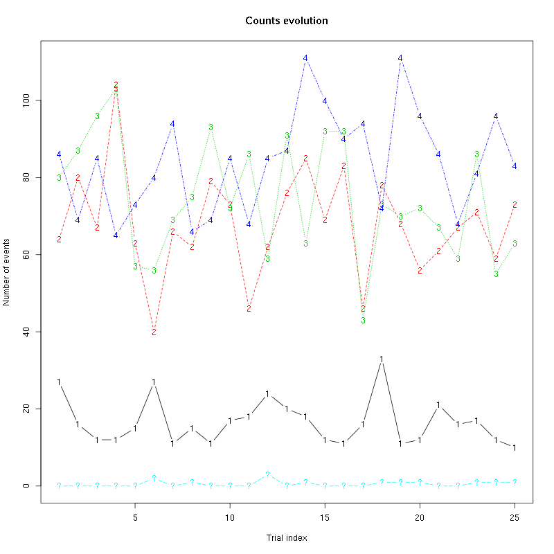
Figure 14: Evolution of the number of events attributed to each unit (1 to 4) or unclassified ("?") during the 25 trials of Hexanal for tetrode D2.
The waveform evolution is:
waveform_evolution(a_Hexanal_tetD2,threshold_factor)
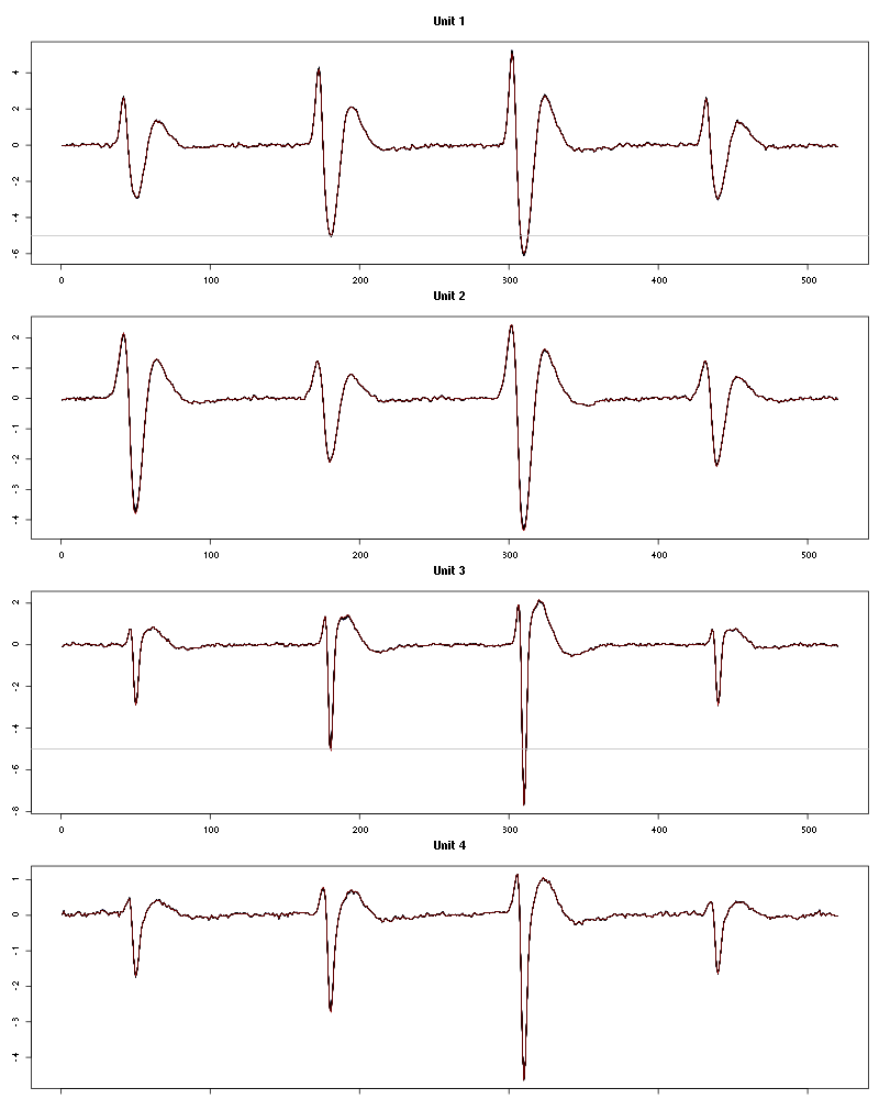
Figure 15: Evolution of the templates of each unit during the 25 trials of Hexanal for tetrode D2.
The observed counting processes, inter spike intervals densities and raster plots are:
cp_isi_raster(a_Hexanal_tetD2)
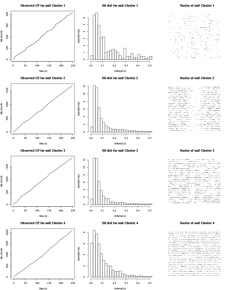
Figure 16: Observed counting processes, empirical inter spike interval distributions and raster plots for Hexanal.
5.3 Save results
Before analyzing the next set of trials we save the output of smt to disk with:
save(a_Hexanal_tetD2,
     file=paste0("tetD2_analysis/tetD2_","Hexanal","_summary_obj.rda"))
We write to disk the spike trains in text mode:
for (c_idx in 1:length(a_Hexanal_tetD2$spike_trains))
    cat(a_Hexanal_tetD2$spike_trains[[c_idx]],
        file=paste0("locust20000421_spike_trains/locust20000421_Hexanal_tetD2_u",c_idx,".txt"),sep="\n")
6 25 trials with Cis-3-Hexen-1-ol
We will carry out an analysis of the 25 trials from Cis-3-Hexen-1-ol.
6.1 Do the job
We do not print out the output to save space.
a_Cis_3_Hexen_1_ol_tetD2=smt(stim_name="Cis-3-Hexen-1-ol",
                             centers=a_Hexanal_tetD2$centers,
                             counts=a_Hexanal_tetD2$counts)
6.2 Diagnostic plots
The counts evolution is:
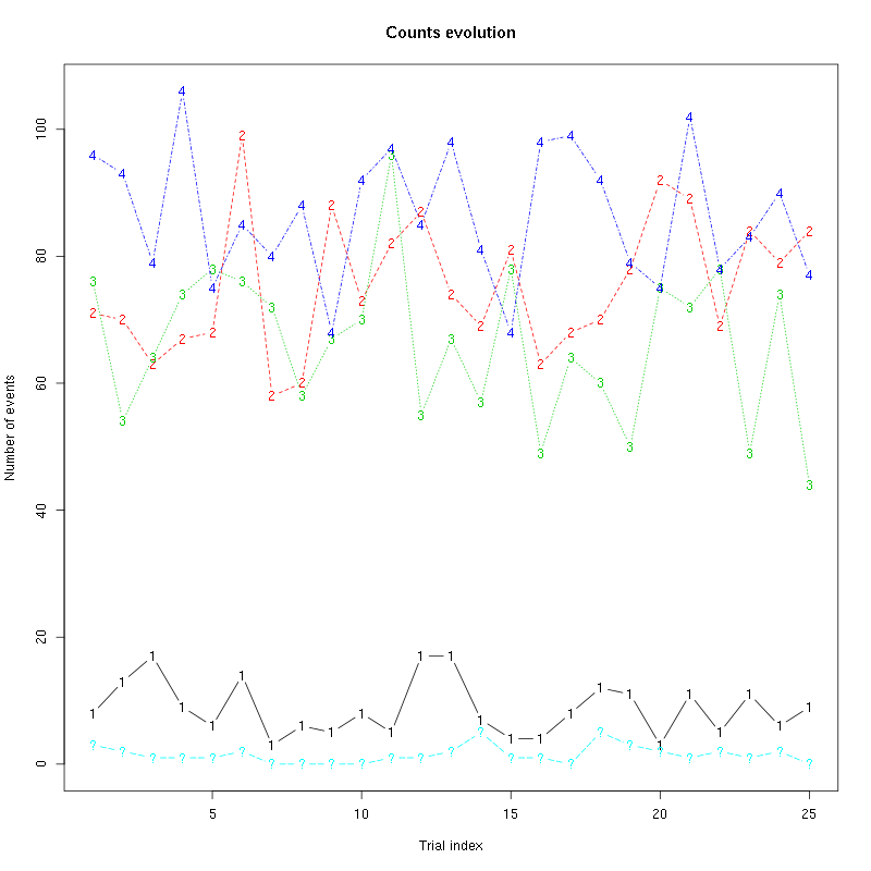
Figure 17: Evolution of the number of events attributed to each unit (1 to 4) or unclassified ("?") during the 30 trials of Cis-3-Hexen-1-ol for tetrode D2.
The waveform evolution is:
waveform_evolution(a_Cis_3_Hexen_1_ol_tetD2,threshold_factor)

Figure 18: Evolution of the templates of each unit during the 25 trials of Cis-3-Hexen-1-ol for stereode Ca.
The observed counting processes, inter spike intervals densities and raster plots are:
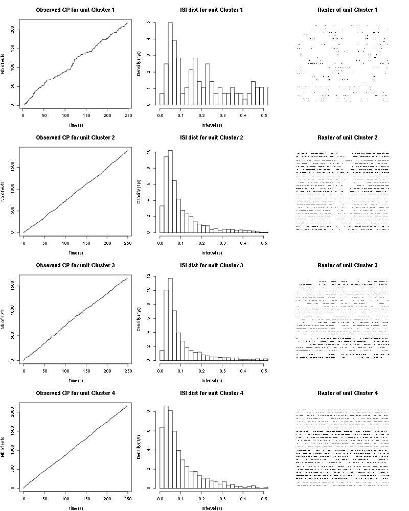
Figure 19: Observed counting processes, empirical inter spike interval distributions and raster plots for Cis-3-Hexen-1-ol.
6.3 Save results
Before analyzing the next set of trials we save the output of smt to disk with:
save(a_Cis_3_Hexen_1_ol_tetD2,
     file=paste0("tetD2_analysis/tetD2_","Cis-3-Hexen-1-ol","_summary_obj.rda"))
We write to disk the spike trains in text mode:
for (c_idx in 1:length(a_Cis_3_Hexen_1_ol_tetD2$spike_trains))
    if (!is.null(a_Cis_3_Hexen_1_ol_tetD2$spike_trains[[c_idx]]))
        cat(a_Cis_3_Hexen_1_ol_tetD2$spike_trains[[c_idx]],
	    file=paste0("locust20000421_spike_trains/locust20000421_Cis-3-Hexen-1-ol_tetD2_u",c_idx,".txt"),sep="\n")
7 25 trials with Trans-2-Hexen-1-ol
We will carry out an analysis of the 25 trials from Trans-2-Hexen-1-ol.
7.1 Do the job
stim_name = "Trans-2-Hexen-1-ol"
a_Trans_2_Hexen_1_ol_tetD2=smt(stim_name=stim_name,
                               centers=a_Cis_3_Hexen_1_ol_tetD2$centers,
                               counts=a_Cis_3_Hexen_1_ol_tetD2$counts)
7.2 Diagnostic plots
The counts evolution is:
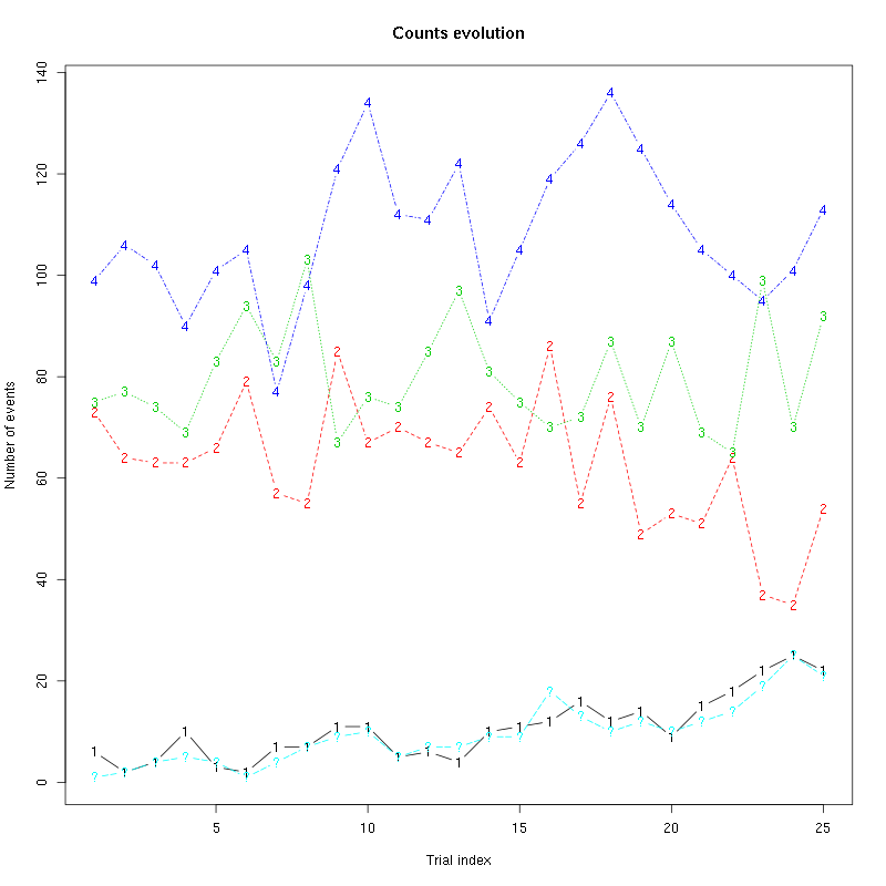
Figure 20: Evolution of the number of events attributed to each unit (1 to 4) or unclassified ("?") during the 25 trials of Trans-2-Hexen-1-ol for tetrodeD2.
The waveform evolution is:
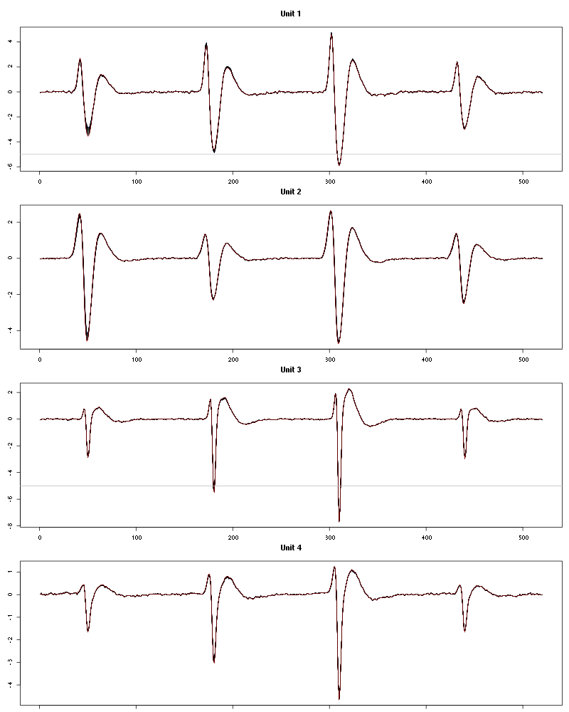
Figure 21: Evolution of the templates of each unit during the 25 trials of Trans-2-Hexen-1-ol for tetrodeD2.
The observed counting processes, inter spike intervals densities and raster plots are:
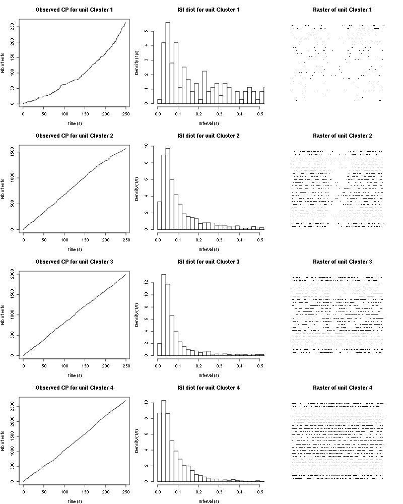
Figure 22: Observed counting processes, empirical inter spike interval distributions and raster plots for Trans-2-Hexen-1-ol.
7.3 Save results
Before analyzing the next set of trials we save the output of smt to disk with:
save(a_Trans_2_Hexen_1_ol_tetD2,
     file=paste0("tetD2_analysis/tetD2_",stim_name,"_summary_obj.rda"))
We write to disk the spike trains in text mode:
for (c_idx in 1:length(a_Trans_2_Hexen_1_ol_tetD2$spike_trains))
    if (!is.null(a_Trans_2_Hexen_1_ol_tetD2$spike_trains[[c_idx]]))
        cat(a_Trans_2_Hexen_1_ol_tetD2$spike_trains[[c_idx]],file=paste0("locust20000421_spike_trains/locust20000421_Trans-2-Hexen-1-ol_tetD2_u",c_idx,".txt"),sep="\n")
8 25 trials with 1-Hexen-3-ol
We will carry out an analysis of the 25 trials from 1-Hexen-3-ol.
8.1 Do the job
stim_name = "1-Hexen-3-ol"
a_1_Hexen_3_ol_tetD2=smt(stim_name=stim_name,
                         centers=a_Trans_2_Hexen_1_ol_tetD2$centers,
                         counts=a_Trans_2_Hexen_1_ol_tetD2$counts)
8.2 Diagnostic plots
The counts evolution is:
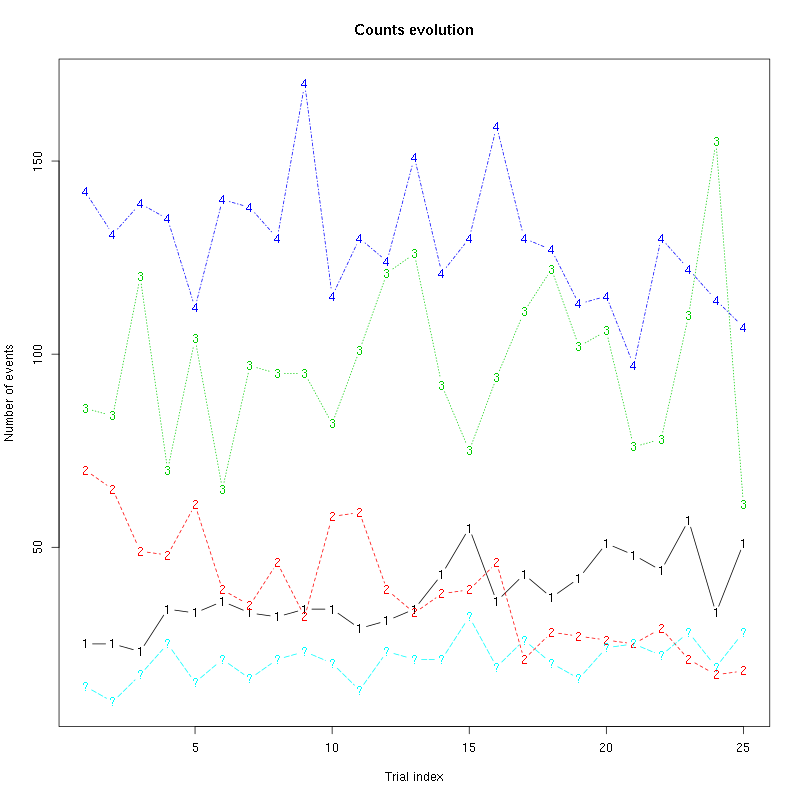
Figure 23: Evolution of the number of events attributed to each unit (1 to 4) or unclassified ("?") during the 25 trials of 1-Hexen-3-ol for tetrodeD2.
The waveform evolution is:
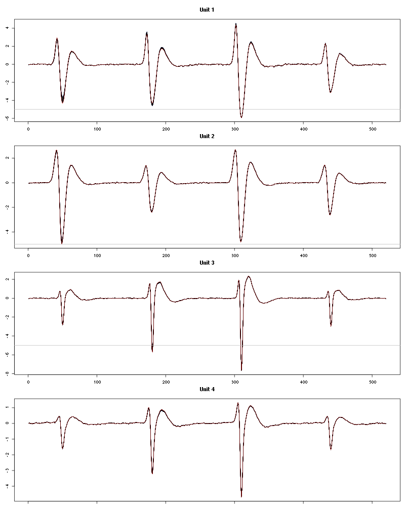
Figure 24: Evolution of the templates of each unit during the 25 trials of 1-Hexen-3-ol for tetrodeD2.
The observed counting processes, inter spike intervals densities and raster plots are:
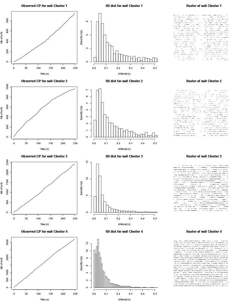
Figure 25: Observed counting processes, empirical inter spike interval distributions and raster plots for 1-Hexen-3-ol.
8.3 Save results
Before analyzing the next set of trials we save the output of smt to disk with:
save(a_1_Hexen_3_ol_tetD2,
     file=paste0("tetD2_analysis/tetD2_",stim_name,"_summary_obj.rda"))
We write to disk the spike trains in text mode:
for (c_idx in 1:length(a_1_Hexen_3_ol_tetD2$spike_trains))
    if (!is.null(a_1_Hexen_3_ol_tetD2$spike_trains[[c_idx]]))
        cat(a_1_Hexen_3_ol_tetD2$spike_trains[[c_idx]],file=paste0("locust20000421_spike_trains/locust20000421_1-Hexen-3-ol_tetD2_u",c_idx,".txt"),sep="\n")
9 25 trials with 3-Pentanone
We will carry out an analysis of the 25 trials from 3-Pentanone.
9.1 Do the job
stim_name = "3-Pentanone"
a_3_Pentanone_tetD2=smt(stim_name=stim_name,
                        centers=a_1_Hexen_3_ol_tetD2$centers,
                        counts=a_1_Hexen_3_ol_tetD2$counts)
9.2 Diagnostic plots
The counts evolution is:
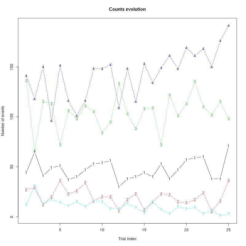
Figure 26: Evolution of the number of events attributed to each unit (1 to 4) or unclassified ("?") during the 25 trials of 3-Pentanone for tetrodeD2.
The waveform evolution is:
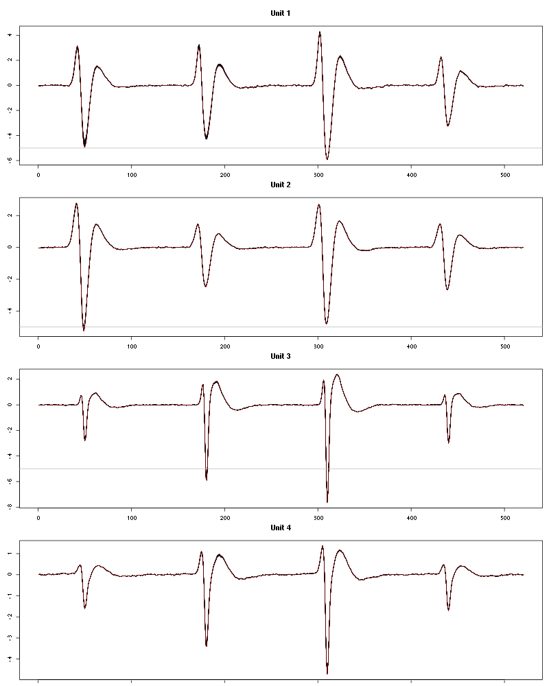
Figure 27: Evolution of the templates of each of the first four units during the 25 trials of 3-Pentanone for tetrodeD2.
The observed counting processes, inter spike intervals densities and raster plots are:
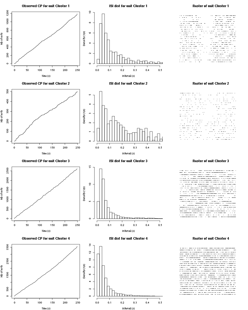
Figure 28: Observed counting processes, empirical inter spike interval distributions and raster plots for 3-Pentanone.
9.3 Save results
Before analyzing the next set of trials we save the output of smt to disk with:
save(a_3_Pentanone_tetD2,
     file=paste0("tetD2_analysis/tetD2_",stim_name,"_summary_obj.rda"))
We write to disk the spike trains in text mode:
for (c_idx in 1:length(a_3_Pentanone_tetD2$spike_trains))
    if (!is.null(a_3_Pentanone_tetD2$spike_trains[[c_idx]]))
        cat(a_3_Pentanone_tetD2$spike_trains[[c_idx]],file=paste0("locust20000421_spike_trains/locust20000421_3-Pentanone_tetD2_u",c_idx,".txt"),sep="\n")
10 25 trials with 1-Heptanol
We will carry out an analysis of the 25 trials from 1-Heptanol.
10.1 Do the job
stim_name = "1-Heptanol"
a_1_Heptanol_tetD2=smt(stim_name=stim_name,
                       centers=a_3_Pentanone_tetD2$centers,
                       counts=a_3_Pentanone_tetD2$counts)
10.2 Diagnostic plots
The counts evolution is:
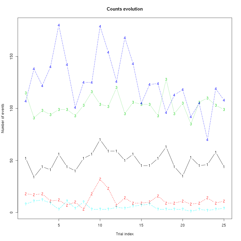
Figure 29: Evolution of the number of events attributed to each unit (1 to 4) or unclassified ("?") during the 25 trials of 1-Heptanol for tetrodeD2.
The waveform evolution is:
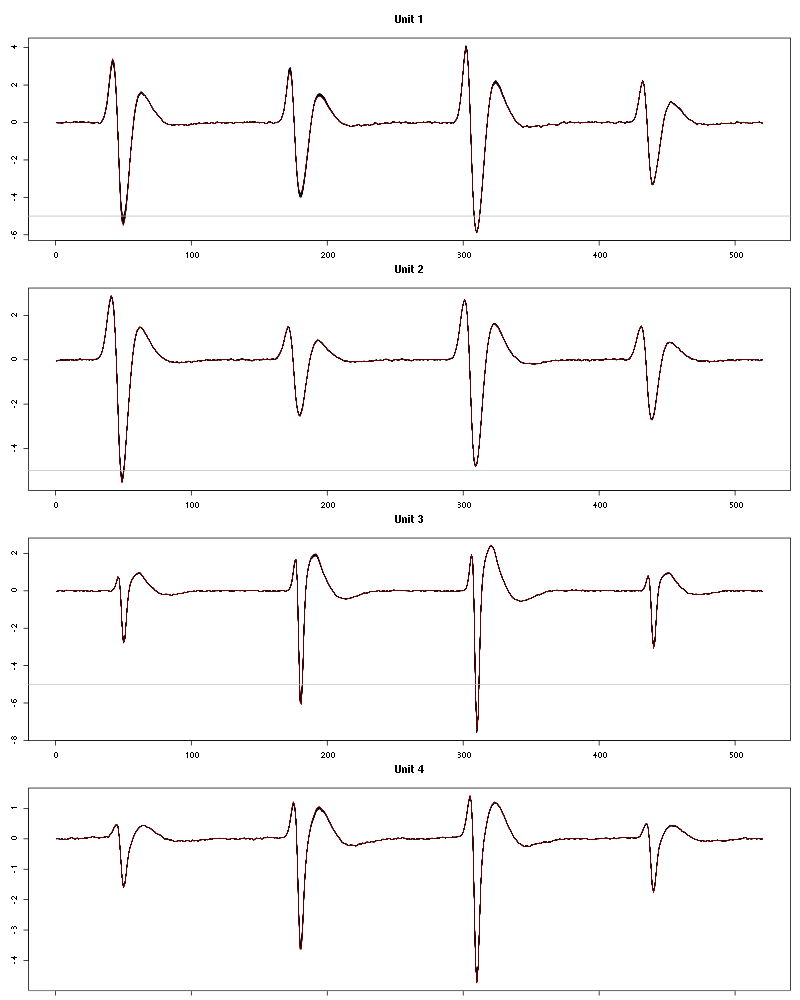
Figure 30: Evolution of the templates of each of the first four units during the 25 trials of 1-Heptanol for tetrodeD2.
The observed counting processes, inter spike intervals densities and raster plots are:
cp_isi_raster(a_1_Heptanol_tetD2)
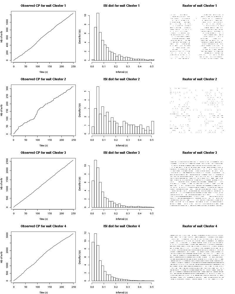
Figure 31: Observed counting processes, empirical inter spike interval distributions and raster plots for 1-Heptanol.
10.3 Save results
Before analyzing the next set of trials we save the output of smt to disk with:
save(a_1_Heptanol_tetD2,
     file=paste0("tetD2_analysis/tetD2_",stim_name,"_summary_obj.rda"))
We write to disk the spike trains in text mode:
for (c_idx in 1:length(a_1_Heptanol_tetD2$spike_trains))
    if (!is.null(a_1_Heptanol_tetD2$spike_trains[[c_idx]]))
        cat(a_1_Heptanol_tetD2$spike_trains[[c_idx]],file=paste0("locust20000421_spike_trains/locust20000421_1-Heptanol_tetD2_u",c_idx,".txt"),sep="\n")
11 25 trials with 1-Octanol (10^-0) first
We will carry out an analysis of the 25 trials from 1-Octanol (10^-0) first.
11.1 Do the job
stim_name = "1-Octanol (10^-0) first"
a_1_Octanol_0_tetD2=smt(stim_name=stim_name,
                        centers=a_1_Heptanol_tetD2$centers,
                        counts=a_1_Heptanol_tetD2$counts)
11.2 Diagnostic plots
The counts evolution is:
 first-count-evolution-tetD2.png)
Figure 32: Evolution of the number of events attributed to each unit (1 to 4) or unclassified ("?") during the 25 trials of 1-Octanol (10^-0) first for tetrodeD2.
The waveform evolution is:
 first-waveform-evolution-tetD2.png)
Figure 33: Evolution of the templates of each of the first four units during the 25 trials of 1-Octanol (10^-0) first for tetrodeD2.
The observed counting processes, inter spike intervals densities and raster plots are:
cp_isi_raster(a_1_Octanol_0_tetD2)
 first-CP-and-ISI-dist-tetD2.png)
Figure 34: Observed counting processes, empirical inter spike interval distributions and raster plots for 1-Octanol (10^-0) first.
11.3 Save results
Before analyzing the next set of trials we save the output of smt to disk with:
save(a_1_Octanol_0_tetD2,
     file=paste0("tetD2_analysis/tetD2_",stim_name,"_summary_obj.rda"))
We write to disk the spike trains in text mode:
for (c_idx in 1:length(a_1_Octanol_0_tetD2$spike_trains))
    if (!is.null(a_1_Octanol_0_tetD2$spike_trains[[c_idx]]))
        cat(a_1_Octanol_0_tetD2$spike_trains[[c_idx]],file=paste0("locust20000421_spike_trains/locust20000421_1-Octanol (10^-0) first_tetD2_u",c_idx,".txt"),sep="\n")
12 25 trials with 2-Heptanone
We will carry out an analysis of the 25 trials from 2-Heptanone.
12.1 Do the job
stim_name = "2-Heptanone"
a_2_Heptanone_tetD2=smt(stim_name=stim_name,
                        centers=a_1_Octanol_0_tetD2$centers,
                        counts=a_1_Octanol_0_tetD2$counts)
12.2 Diagnostic plots
The counts evolution is:
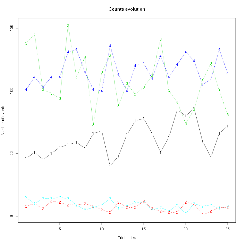
Figure 35: Evolution of the number of events attributed to each unit (1 to 4) or unclassified ("?") during the 25 trials of 2-Heptanone for tetrodeD2.
The waveform evolution is:
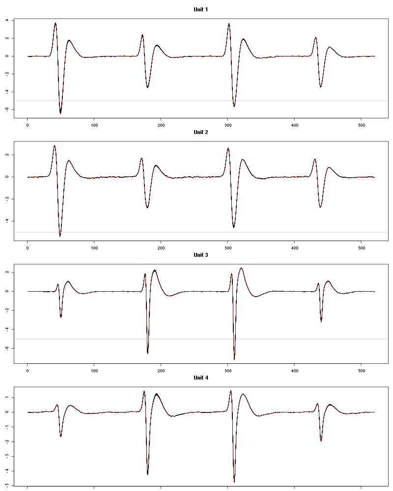
Figure 36: Evolution of the templates of each unit during the 25 trials of 2-Heptanone for tetrodeD2.
The observed counting processes, inter spike intervals densities and raster plots are:
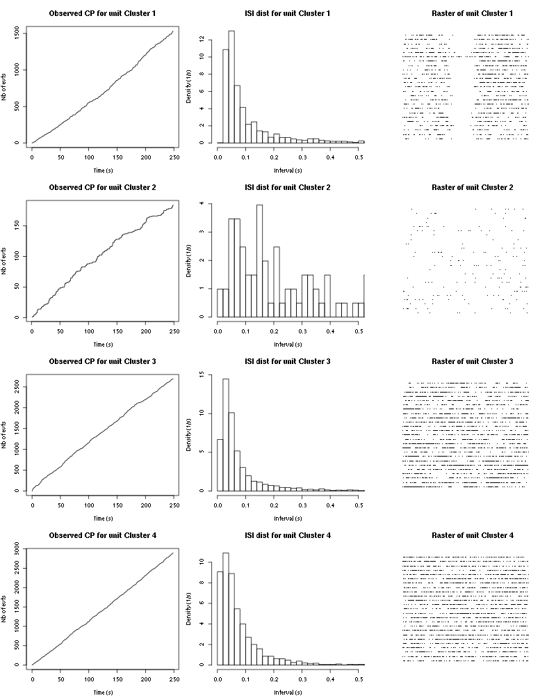
Figure 37: Observed counting processes, empirical inter spike interval distributions and raster plots for 2-Heptanone.
12.3 Save results
Before analyzing the next set of trials we save the output of smt to disk with:
save(a_2_Heptanone_tetD2,
     file=paste0("tetD2_analysis/tetD2_",stim_name,"_summary_obj.rda"))
We write to disk the spike trains in text mode:
for (c_idx in 1:length(a_2_Heptanone_tetD2$spike_trains))
    if (!is.null(a_2_Heptanone_tetD2$spike_trains[[c_idx]]))
        cat(a_2_Heptanone_tetD2$spike_trains[[c_idx]],file=paste0("locust20000421_spike_trains/locust20000421_2-Heptanone_tetD2_u",c_idx,".txt"),sep="\n")
13 25 trials with 3-Heptanone
We will carry out an analysis of the 25 trials from 3-Heptanone.
13.1 Do the job
stim_name = "3-Heptanone"
a_3_Heptanone_tetD2=smt(stim_name=stim_name,
                        centers=a_2_Heptanone_tetD2$centers,
                        counts=a_2_Heptanone_tetD2$counts)
13.2 Diagnostic plots
The counts evolution is:
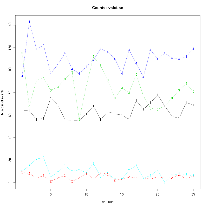
Figure 38: Evolution of the number of events attributed to each unit (1 to 4) or unclassified ("?") during the 25 trials of 3-Heptanone for tetrodeD2.
The waveform evolution is:
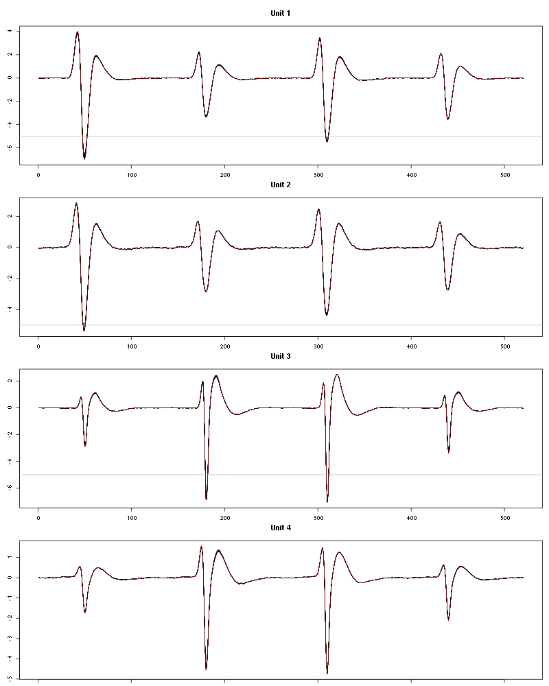
Figure 39: Evolution of the templates of each unit during the 25 trials of 3-Heptanone for tetrodeD2.
The observed counting processes, inter spike intervals densities and raster plots are:
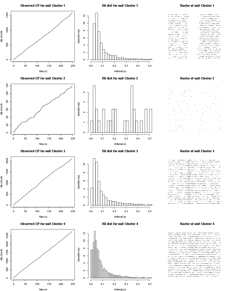
Figure 40: Observed counting processes, empirical inter spike interval distributions and raster plots for 3-Heptanone.
13.3 Save results
Before analyzing the next set of trials we save the output of smt to disk with:
save(a_3_Heptanone_tetD2,
     file=paste0("tetD2_analysis/tetD2_",stim_name,"_summary_obj.rda"))
We write to disk the spike trains in text mode:
for (c_idx in 1:length(a_3_Heptanone_tetD2$spike_trains))
    if (!is.null(a_3_Heptanone_tetD2$spike_trains[[c_idx]]))
        cat(a_3_Heptanone_tetD2$spike_trains[[c_idx]],file=paste0("locust20000421_spike_trains/locust20000421_3-Heptanone_tetD2_u",c_idx,".txt"),sep="\n")
14 25 trials with Citral
We will carry out an analysis of the 25 trials from Citral.
14.1 Do the job
stim_name = "Citral"
a_Citral_tetD2=smt(stim_name=stim_name,
                   centers=a_3_Heptanone_tetD2$centers,
                   counts=a_3_Heptanone_tetD2$counts)
14.2 Diagnostic plots
The counts evolution is:
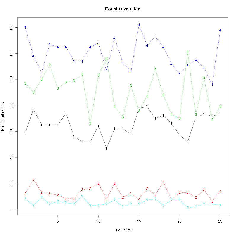
Figure 41: Evolution of the number of events attributed to each unit (1 to 4) or unclassified ("?") during the 25 trials of Citral for tetrodeD2.
The waveform evolution is:
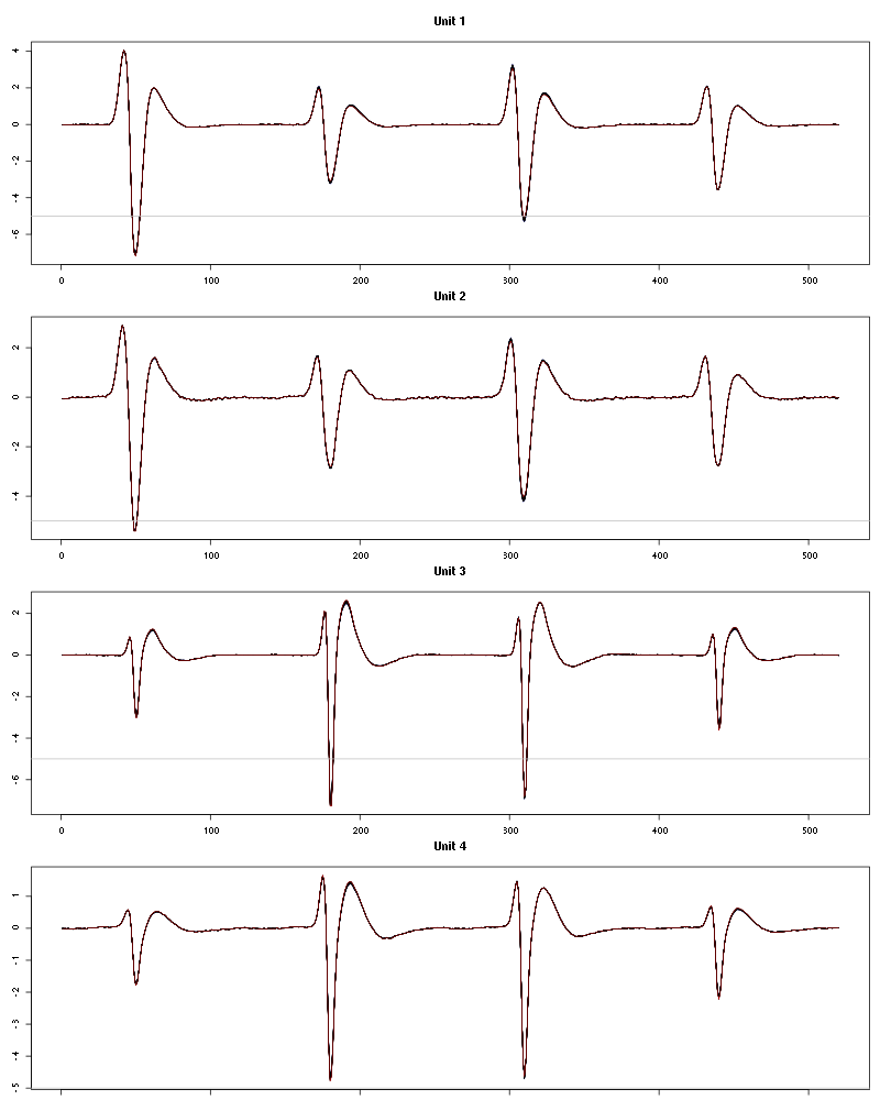
Figure 42: Evolution of the templates of each unit during the 25 trials of Citral for tetrodeD2.
The observed counting processes, inter spike intervals densities and raster plots are:
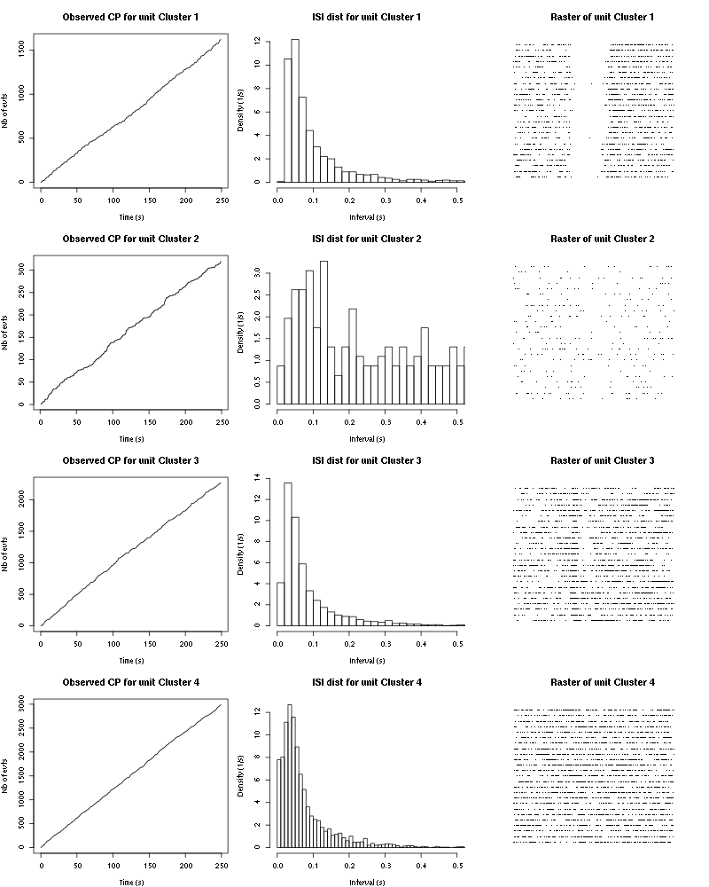
Figure 43: Observed counting processes, empirical inter spike interval distributions and raster plots for Citral.
14.3 Save results
Before analyzing the next set of trials we save the output of smt to disk with:
save(a_Citral_tetD2,
     file=paste0("tetD2_analysis/tetD2_",stim_name,"_summary_obj.rda"))
We write to disk the spike trains in text mode:
for (c_idx in 1:length(a_Citral_tetD2$spike_trains))
    if (!is.null(a_Citral_tetD2$spike_trains[[c_idx]]))
        cat(a_Citral_tetD2$spike_trains[[c_idx]],file=paste0("locust20000421_spike_trains/locust20000421_Citral_tetD2_u",c_idx,".txt"),sep="\n")
15 25 trials with Apple
We will carry out an analysis of the 25 trials from Apple.
15.1 Do the job
stim_name = "Apple"
a_Apple_tetD2=smt(stim_name=stim_name,
                  centers=a_Citral_tetD2$centers,
                  counts=a_Citral_tetD2$counts)
15.2 Diagnostic plots
The counts evolution is:
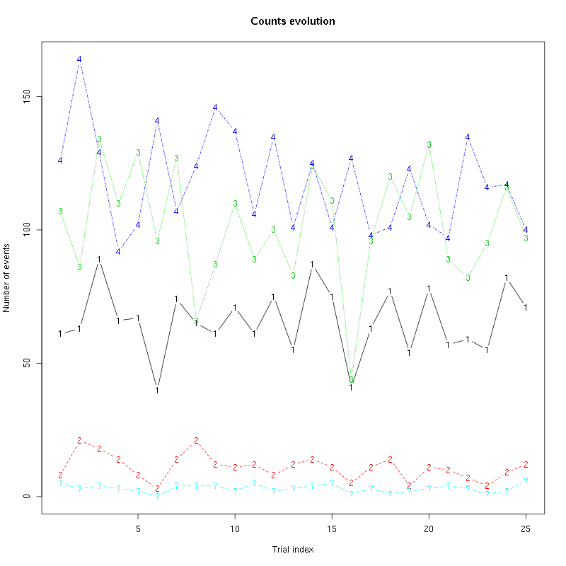
Figure 44: Evolution of the number of events attributed to each unit (1 to 4) or unclassified ("?") during the 25 trials of Apple for tetrodeD2.
The waveform evolution is:
waveform_evolution(a_Apple_tetD2,threshold_factor)
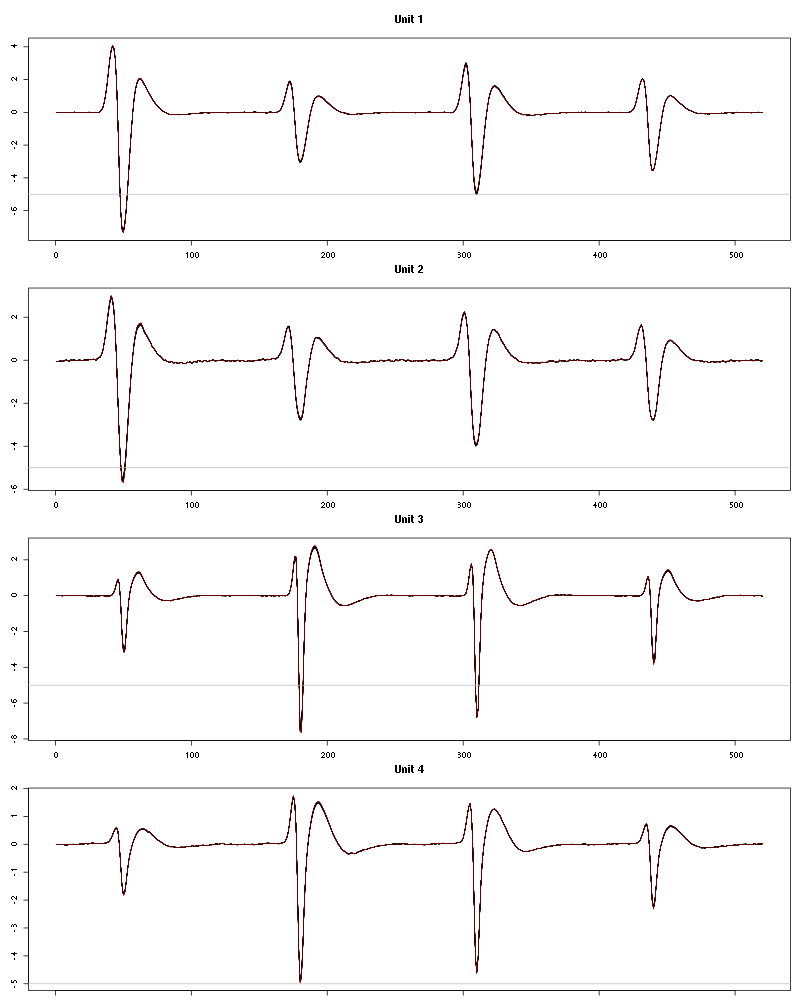
Figure 45: Evolution of the templates of each unit during the 25 trials of Apple for tetrodeD2.
The observed counting processes, inter spike intervals densities and raster plots are:
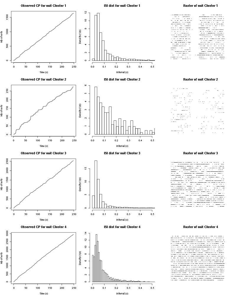
Figure 46: Observed counting processes, empirical inter spike interval distributions and raster plots for Apple.
15.3 Save results
Before analyzing the next set of trials we save the output of smt to disk with:
save(a_Apple_tetD2s,
     file=paste0("tetD2_analysis/tetD2_",stim_name,"_summary_obj.rda"))
We write to disk the spike trains in text mode:
for (c_idx in 1:length(a_Apple_tetD2$spike_trains))
    if (!is.null(a_Apple_tetD2$spike_trains[[c_idx]]))
        cat(a_Apple_tetD2$spike_trains[[c_idx]],file=paste0("locust20000421_spike_trains/locust20000421_Apple_tetD2_u",c_idx,".txt"),sep="\n")
16 25 trials with Mint
We will carry out an analysis of the 25 trials from Mint.
16.1 Do the job
stim_name = "Mint"
a_Mint_tetD2=smt(stim_name=stim_name,
                 centers=a_Apple_tetD2$centers,
                 counts=a_Apple_tetD2$counts)
16.2 Diagnostic plots
The counts evolution is:
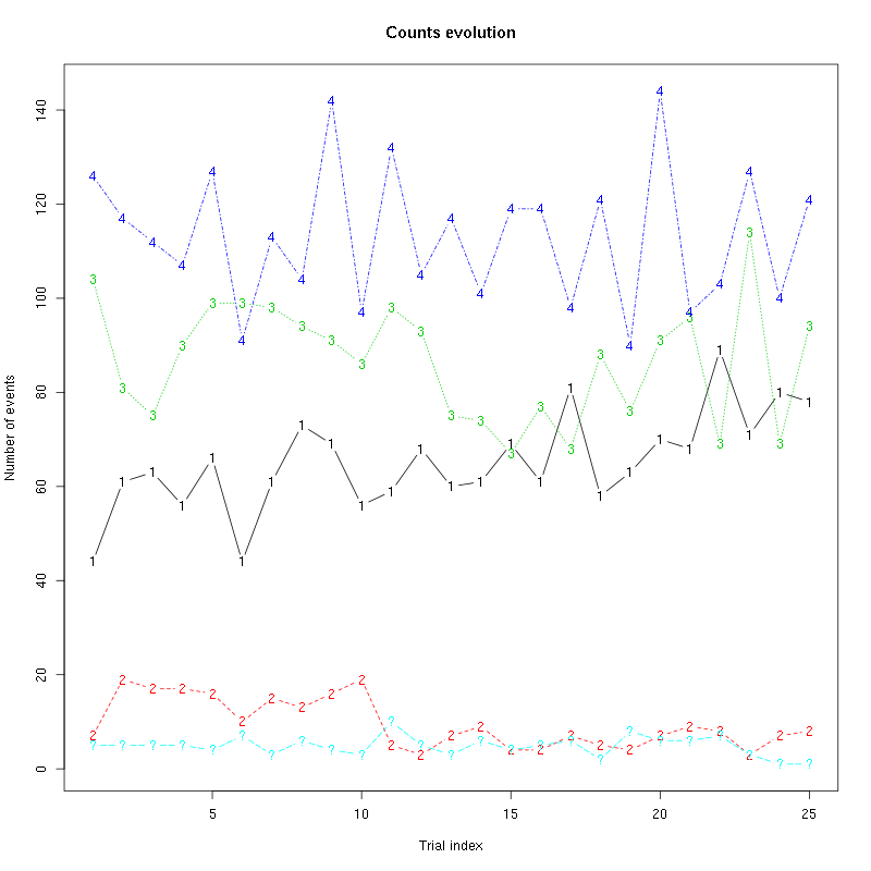
Figure 47: Evolution of the number of events attributed to each unit (1 to 4) or unclassified ("?") during the 25 trials of Mint for tetrodeD2.
The waveform evolution is:
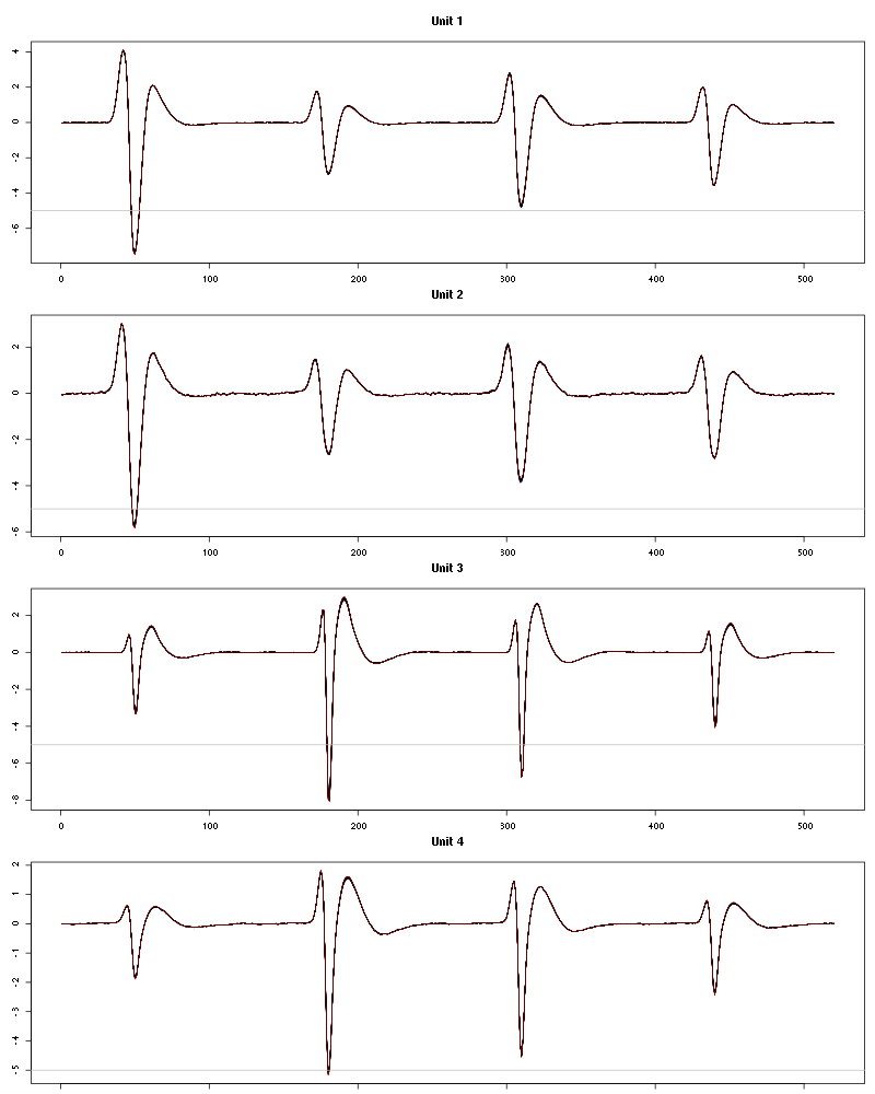
Figure 48: Evolution of the templates of each unit during the 25 trials of Mint for tetrodeD2.
The observed counting processes, inter spike intervals densities and raster plots are:
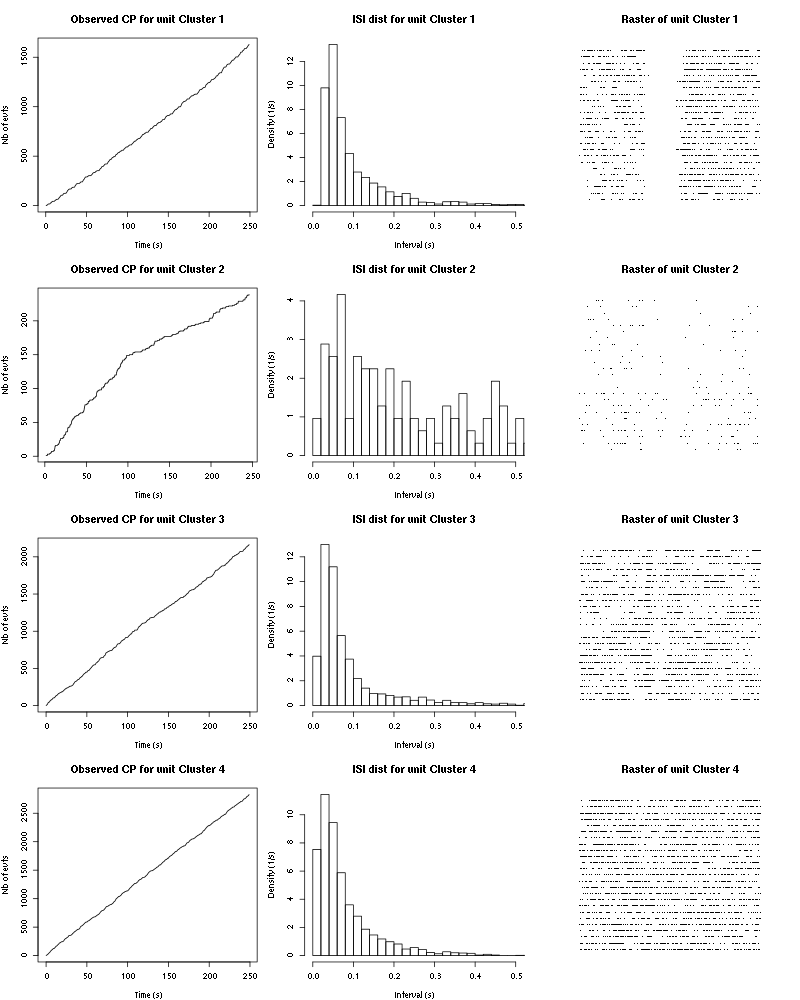
Figure 49: Observed counting processes, empirical inter spike interval distributions and raster plots for Mint.
16.3 Save results
Before analyzing the next set of trials we save the output of smt to disk with:
save(a_Mint_tetD2,
     file=paste0("tetD2_analysis/tetD2_",stim_name,"_summary_obj.rda"))
We write to disk the spike trains in text mode:
for (c_idx in 1:length(a_Mint_sterC$spike_trains))
    if (!is.null(a_Mint_sterC$spike_trains[[c_idx]]))
        cat(a_Mint_sterC$spike_trains[[c_idx]],file=paste0("locust20000421_spike_trains/locust20000421_Mint_tetD2_u",c_idx,".txt"),sep="\n")
17 25 trials with Strawberry
We will carry out an analysis of the 25 trials from Strawberry.
17.1 Do the job
stim_name = "Strawberry"
a_Strawberry_tetD2=smt(stim_name=stim_name,
                       centers=a_Mint_tetD2$centers,
                       counts=a_Mint_tetD2$counts)
17.2 Diagnostic plots
The counts evolution is:
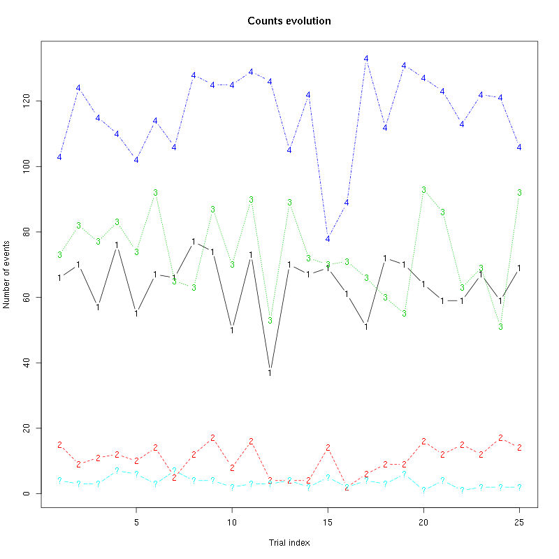
Figure 50: Evolution of the number of events attributed to each unit (1 to 4) or unclassified ("?") during the 25 trials of Strawberry for tetrodeD2.
The waveform evolution is:
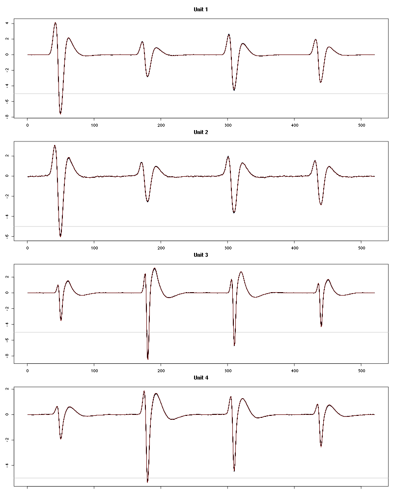
Figure 51: Evolution of the templates of each unit during the 25 trials of Strawberry for tetrodeD2.
The observed counting processes, inter spike intervals densities and raster plots are:
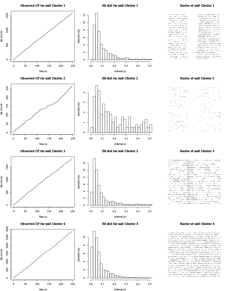
Figure 52: Observed counting processes, empirical inter spike interval distributions and raster plots for Strawberry.
17.3 Save results
Before analyzing the next set of trials we save the output of smt to disk with:
save(a_Strawberry_tetD2,
     file=paste0("tetD2_analysis/tetD2_",stim_name,"_summary_obj.rda"))
We write to disk the spike trains in text mode:
for (c_idx in 1:length(a_Strawberry_sterC$spike_trains))
    if (!is.null(a_Strawberry_sterC$spike_trains[[c_idx]]))
        cat(a_Strawberry_sterC$spike_trains[[c_idx]],file=paste0("locust20000421_spike_trains/locust20000421_Strawberry_tetD2_u",c_idx,".txt"),sep="\n")
18 25 trials with Amyl Acetate
We will carry out an analysis of the 25 trials from Amyl Acetate.
18.1 Do the job
stim_name = "Amyl Acetate"
a_Amyl_Acetate_tetD2=smt(stim_name=stim_name,
                         centers=a_Strawberry_tetD2$centers,
                         counts=a_Strawberry_tetD2$counts)
18.2 Diagnostic plots
The counts evolution is:
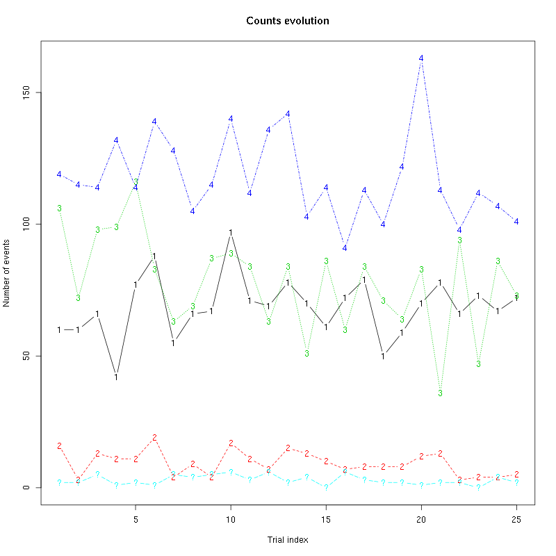
Figure 53: Evolution of the number of events attributed to each unit (1 to 4) or unclassified ("?") during the 25 trials of Amyl Acetate for tetrodeD2.
The waveform evolution is:
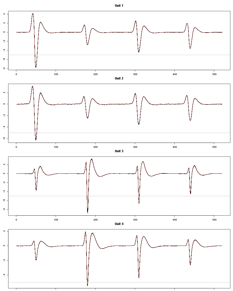
Figure 54: Evolution of the templates of each unit during the 25 trials of Amyl Acetate for tetrodeD2.
The observed counting processes, inter spike intervals densities and raster plots are:
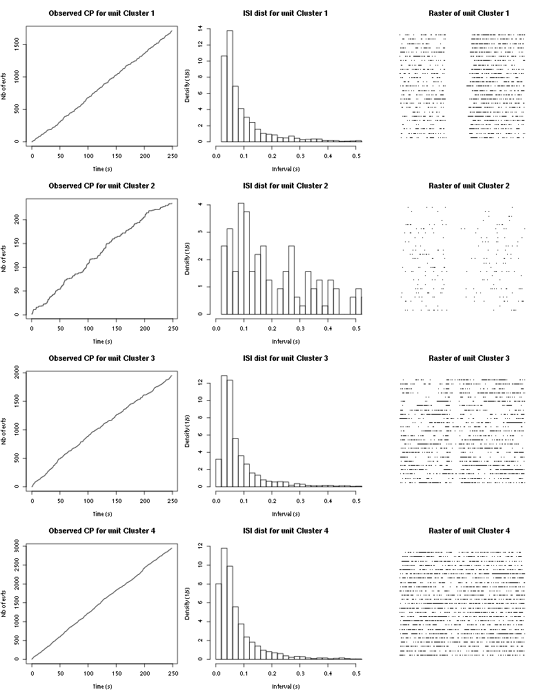
Figure 55: Observed counting processes, empirical inter spike interval distributions and raster plots for Amyl Acetate.
18.3 Save results
Before analyzing the next set of trials we save the output of smt to disk with:
save(a_Amyl_Acetate_tetD2,
     file=paste0("tetD2_analysis/tetD2_",stim_name,"_summary_obj.rda"))
We write to disk the spike trains in text mode:
for (c_idx in 1:length(a_Amyl_Acetate_tetD2$spike_trains))
    if (!is.null(a_Amyl_Acetate_tetD2$spike_trains[[c_idx]]))
        cat(a_Amyl_Acetate_tetD2$spike_trains[[c_idx]],file=paste0("locust20000421_spike_trains/locust20000421_Amyl Acetate_tetD2_u",c_idx,".txt"),sep="\n")
19 25 trials with Octaldehyde
We will carry out an analysis of the 25 trials from Octaldehyde.
19.1 Do the job
stim_name = "Octaldehyde"
a_Octaldehyde_tetD2=smt(stim_name=stim_name,
                        centers=a_Amyl_Acetate_tetD2$centers,
                        counts=a_Amyl_Acetate_tetD2$counts)
19.2 Diagnostic plots
The counts evolution is:
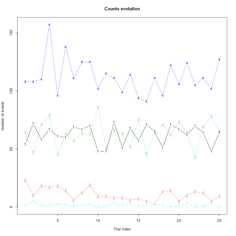
Figure 56: Evolution of the number of events attributed to each unit (1 to 4) or unclassified ("?") during the 25 trials of Octaldehyde for tetrodeD2.
The waveform evolution is:
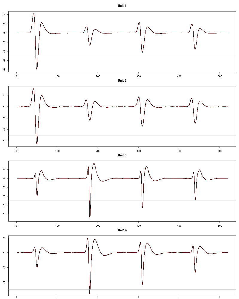
Figure 57: Evolution of the templates of each unit during the 25 trials of Octaldehyde for tetrodeD2.
The observed counting processes, inter spike intervals densities and raster plots are:
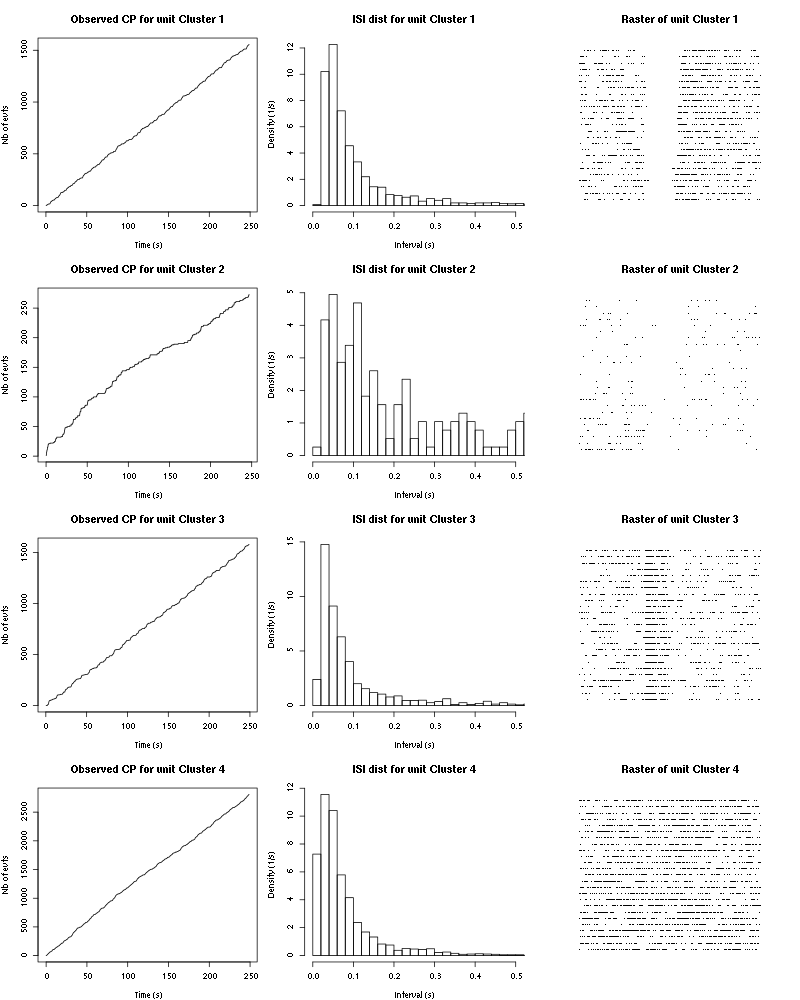
Figure 58: Observed counting processes, empirical inter spike interval distributions and raster plots for Octaldehyde.
19.3 Save results
Before analyzing the next set of trials we save the output of smt to disk with:
save(a_Octaldehyde_tetD2,
     file=paste0("tetD2_analysis/tetD2_",stim_name,"_summary_obj.rda"))
We write to disk the spike trains in text mode:
for (c_idx in 1:length(a_Octaldehyde_tetD2$spike_trains))
    if (!is.null(a_Octaldehyde_tetD2$spike_trains[[c_idx]]))
        cat(a_Octaldehyde_tetD2$spike_trains[[c_idx]],file=paste0("locust20000421_spike_trains/locust20000421_Octaldehyde_tetD2_u",c_idx,".txt"),sep="\n")
20 25 trials with 1-Octanol (10^-5)
We will carry out an analysis of the 25 trials from 1-Octanol (10^-5).
20.1 Do the job
stim_name = "1-Octanol (10^-5)"
a_1_Octanol_5_tetD2=smt(stim_name=stim_name,
                        centers=a_Octaldehyde_tetD2$centers,
                        counts=a_Octaldehyde_tetD2$counts)
20.2 Diagnostic plots
The counts evolution is:
-count-evolution-tetD2.png)
Figure 59: Evolution of the number of events attributed to each unit (1 to 4) or unclassified ("?") during the 25 trials of 1-Octanol (10^-5) for tetrodeD2.
The waveform evolution is:
-waveform-evolution-tetD2.png)
Figure 60: Evolution of the templates of each unit during the 25 trials of 1-Octanol (10^-5) for tetrodeD2.
The observed counting processes, inter spike intervals densities and raster plots are:
-CP-and-ISI-dist-tetD2.png)
Figure 61: Observed counting processes, empirical inter spike interval distributions and raster plots for 1-Octanol (10^-5).
20.3 Save results
Before analyzing the next set of trials we save the output of smt to disk with:
save(a_1_Octanol_5_tetD2,
     file=paste0("tetD2_analysis/tetD2_",stim_name,"_summary_obj.rda"))
We write to disk the spike trains in text mode:
for (c_idx in 1:length(a_1_Octanol_5_tetD2$spike_trains))
    if (!is.null(a_1_Octanol_5_tetD2$spike_trains[[c_idx]]))
        cat(a_1_Octanol_5_tetD2$spike_trains[[c_idx]],file=paste0("locust20000421_spike_trains/locust20000421_1-Octanol (10^-5)_tetD2_u",c_idx,".txt"),sep="\n")
21 25 trials with 1-Octanol (10^-4)
We will carry out an analysis of the 25 trials from 1-Octanol (10^-4).
21.1 Do the job
stim_name = "1-Octanol (10^-4)"
a_1_Octanol_4_tetD2=smt(stim_name=stim_name,
                        centers=a_1_Octanol_5_tetD2$centers,
                        counts=a_1_Octanol_5_tetD2$counts)
21.2 Diagnostic plots
The counts evolution is:
-count-evolution-tetD2.png)
Figure 62: Evolution of the number of events attributed to each unit (1 to 4) or unclassified ("?") during the 25 trials of 1-Octanol (10^-4) for tetrodeD2.
The waveform evolution is:
-waveform-evolution-tetD2.png)
Figure 63: Evolution of the templates of each unit during the 25 trials of 1-Octanol (10^-4) for tetrodeD2.
The observed counting processes, inter spike intervals densities and raster plots are:
-CP-and-ISI-dist-tetD2.png)
Figure 64: Observed counting processes, empirical inter spike interval distributions and raster plots for 1-Octanol (10^-4).
21.3 Save results
Before analyzing the next set of trials we save the output of smt to disk with:
save(a_1_Octanol_4_tetD2,
     file=paste0("tetD2_analysis/tetD2_",stim_name,"_summary_obj.rda"))
We write to disk the spike trains in text mode:
for (c_idx in 1:length(a_1_Octanol_4_tetD2$spike_trains))
    if (!is.null(a_1_Octanol_4_tetD2$spike_trains[[c_idx]]))
        cat(a_1_Octanol_4_tetD2$spike_trains[[c_idx]],file=paste0("locust20000421_spike_trains/locust20000421_1-Octanol (10^-4)_tetD2_u",c_idx,".txt"),sep="\n")
22 25 trials with 1-Octanol (10^-3)
We will carry out an analysis of the 25 trials from 1-Octanol (10^-3).
22.1 Do the job
stim_name = "1-Octanol (10^-3)"
a_1_Octanol_3_tetD2=smt(stim_name=stim_name,
                        centers=a_1_Octanol_4_tetD2$centers,
                        counts=a_1_Octanol_4_tetD2$counts)
22.2 Diagnostic plots
The counts evolution is:
-count-evolution-tetD2.png)
Figure 65: Evolution of the number of events attributed to each unit (1 to 4) or unclassified ("?") during the 25 trials of 1-Octanol (10^-3) for tetrodeD2.
The waveform evolution is:
-waveform-evolution-tetD2.png)
Figure 66: Evolution of the templates of each unit during the 25 trials of 1-Octanol (10^-3) for tetrodeD2.
The observed counting processes, inter spike intervals densities and raster plots are:
-CP-and-ISI-dist-tetD2.png)
Figure 67: Observed counting processes, empirical inter spike interval distributions and raster plots for 1-Octanol (10^-3).
22.3 Save results
Before analyzing the next set of trials we save the output of smt to disk with:
save(a_1_Octanol_3_tetD2,
     file=paste0("tetD2_analysis/tetD2_",stim_name,"_summary_obj.rda"))
We write to disk the spike trains in text mode:
for (c_idx in 1:length(a_1_Octanol_3_tetD2$spike_trains))
    if (!is.null(a_1_Octanol_3_tetD2$spike_trains[[c_idx]]))
        cat(a_1_Octanol_3_tetD2$spike_trains[[c_idx]],file=paste0("locust20000421_spike_trains/locust20000421_1-Octanol (10^-3)_tetD2_u",c_idx,".txt"),sep="\n")
23 25 trials with 1-Octanol (10^-2)
We will carry out an analysis of the 25 trials from 1-Octanol (10^-2).
23.1 Do the job
stim_name = "1-Octanol (10^-2)"
a_1_Octanol_2_tetD2=smt(stim_name=stim_name,
                        centers=a_1_Octanol_3_tetD2$centers,
                        counts=a_1_Octanol_3_tetD2$counts)
23.2 Diagnostic plots
The counts evolution is:
-count-evolution-tetD2.png)
Figure 68: Evolution of the number of events attributed to each unit (1 to 4) or unclassified ("?") during the 25 trials of 1-Octanol (10^-2) for tetrodeD2.
The waveform evolution is:
-waveform-evolution-tetD2.png)
Figure 69: Evolution of the templates of each unit during the 25 trials of 1-Octanol (10^-2) for tetrodeD2.
The observed counting processes, inter spike intervals densities and raster plots are:
-CP-and-ISI-dist-tetD2.png)
Figure 70: Observed counting processes, empirical inter spike interval distributions and raster plots for 1-Octanol (10^-2).
23.3 Save results
Before analyzing the next set of trials we save the output of smt to disk with:
save(a_1_Octanol_2_tetD2,
     file=paste0("tetD2_analysis/tetD2_",stim_name,"_summary_obj.rda"))
We write to disk the spike trains in text mode:
for (c_idx in 1:length(a_1_Octanol_2_tetD2$spike_trains))
    if (!is.null(a_1_Octanol_2_tetD2$spike_trains[[c_idx]]))
        cat(a_1_Octanol_2_tetD2$spike_trains[[c_idx]],file=paste0("locust20000421_spike_trains/locust20000421_1-Octanol (10^-2)_tetD2_u",c_idx,".txt"),sep="\n")
24 25 trials with 1-Octanol (10^-1)
We will carry out an analysis of the 25 trials from 1-Octanol (10^-1).
24.1 Do the job
stim_name = "1-Octanol (10^-1)"
a_1_Octanol_1_tetD2=smt(stim_name=stim_name,
                        centers=a_1_Octanol_2_tetD2$centers,
                        counts=a_1_Octanol_2_tetD2$counts)
24.2 Diagnostic plots
The counts evolution is:
-count-evolution-tetD2.png)
Figure 71: Evolution of the number of events attributed to each unit (1 to 4) or unclassified ("?") during the 25 trials of 1-Octanol (10^-1) for tetrodeD2.
The waveform evolution is:
-waveform-evolution-tetD2.png)
Figure 72: Evolution of the templates of each unit during the 25 trials of 1-Octanol (10^-1) for tetrodeD2.
The observed counting processes, inter spike intervals densities and raster plots are:
-CP-and-ISI-dist-tetD2.png)
Figure 73: Observed counting processes, empirical inter spike interval distributions and raster plots for 1-Octanol (10^-1).
24.3 Save results
Before analyzing the next set of trials we save the output of smt to disk with:
save(a_1_Octanol_1_tetD2,
     file=paste0("tetD2_analysis/tetD2_",stim_name,"_summary_obj.rda"))
We write to disk the spike trains in text mode:
for (c_idx in 1:length(a_1_Octanol_1_tetD2$spike_trains))
    if (!is.null(a_1_Octanol_1_tetD2$spike_trains[[c_idx]]))
        cat(a_1_Octanol_1_tetD2$spike_trains[[c_idx]],file=paste0("locust20000421_spike_trains/locust20000421_1-Octanol (10^-1)_tetD2_u",c_idx,".txt"),sep="\n")
25 25 trials with 1-Octanol (10^-0) second
We will carry out an analysis of the 25 trials from 1-Octanol (10^-0) second.
25.1 Do the job
stim_name = "1-Octanol (10^-0) second"
a_1_Octanol_0b_tetD2=smt(stim_name=stim_name,
                         centers=a_1_Octanol_1_tetD2$centers,
                         counts=a_1_Octanol_1_tetD2$counts)
25.2 Diagnostic plots
The counts evolution is:
 second-count-evolution-tetD2.png)
Figure 74: Evolution of the number of events attributed to each unit (1 to 4) or unclassified ("?") during the 25 trials of 1-Octanol (10^-0) second for tetrodeD2.
The waveform evolution is:
 second-waveform-evolution-tetD2.png)
Figure 75: Evolution of the templates of each unit during the 25 trials of 1-Octanol (10^-0) second for tetrodeD2.
The observed counting processes, inter spike intervals densities and raster plots are:
 second-CP-and-ISI-dist-tetD2.png)
Figure 76: Observed counting processes, empirical inter spike interval distributions and raster plots for 1-Octanol (10^-0) second.
25.3 Save results
Before analyzing the next set of trials we save the output of smt to disk with:
save(a_1_Octanol_0b_tetD2,
     file=paste0("tetD2_analysis/tetD2_",stim_name,"_summary_obj.rda"))
We write to disk the spike trains in text mode:
for (c_idx in 1:length(a_1_Octanol_0b_tetD2$spike_trains))
    if (!is.null(a_1_Octanol_0b_tetD2$spike_trains[[c_idx]]))
        cat(a_1_Octanol_0b_tetD2$spike_trains[[c_idx]],file=paste0("locust20000421_spike_trains/locust20000421_1-Octanol (10^-0) second_tetD2_u",c_idx,".txt"),sep="\n")