Sorting data set 20000613 tetrode D (channels 10, 12, 14, 15)

1. Introduction
- 1.1. Getting the data
- 1.2. Getting the code
2. Tetrode D (channels 10, 12, 14, 15) analysis
3. Analyzing a sequence of trials
- 3.1. Create directories were results get saved
- 3.2. Define a "taylored" version of sort_many_trials
4. Systematic analysis of the 50 trials with "pure" Cis-3-Hexen-1-ol
5. 10 remaining trials with Cis-3-Hexen-1-ol diluted 100 times
6. 50 trials with Cis-3-hexen-1-ol diluted 10 times
7. Systematic analysis of the second set of 50 trials with "pure" Cis-3-Hexen-1-ol
8. Systematic analysis of the second set of 20 trials with Cherry

1 Introduction

This is the description of how to do the (spike) sorting of tetrode D (channels 10, 12, 14, 15) from data set locust20000613.

1.1 Getting the data

The data are in file locust20000613.hdf5 located on zenodo and can be downloaded interactivelly with a web browser or by typing at the command line:

wget https://zenodo.org/record/21589/files/locust20000613.hdf5

In the sequel I will assume that R has been started in the directory where the data were downloaded (in other words, the working direcory should be the one containing the data.

The data are in HDF5 format and the easiest way to get them into R is to install the rhdf5 package from Bioconductor. Once the installation is done, the library is loaded into R with:

library(rhdf5)

We can then get a (long and detailed) listing of our data file content with (result not shown):

h5ls("locust20000613.hdf5")

We can get the content of LabBook metadata from the shell with:

h5dump -a "LabBook" locust20000613.hdf5

1.2 Getting the code

The code can be sourced as follows:

source("https://raw.githubusercontent.com/christophe-pouzat/zenodo-locust-datasets-analysis/master/R_Sorting_Code/sorting_with_r.R")

2 Tetrode D (channels 10, 12, 14, 15) analysis

We now want to get our "model", that is a dictionnary of waveforms (one waveform per neuron and per recording site). To that end we are going to use trial_01 (20 s of data) contained in the Cis-3-Hexen-1-ol (10^-0) first Group (in HDF5 jargon).

2.1 Loading the data

So we start by loading the data from channels 10, 12, 14, 15 into R, using the first available trial (50) from the trials with Citral:

lD = get_data(1,"Cis-3-Hexen-1-ol (10^-0) first",
              channels = c("ch10","ch12","ch14","ch15"),
              file="locust20000613.hdf5")
dim(lD)

297620

2.2 Five number summary

We get the Five number summary with:

summary(lD,digits=2)

Min. : 818	Min. : 764	Min. : 372	Min. : 128
1st Qu.:2005	1st Qu.:1959	1st Qu.:2001	1st Qu.:1984
Median :2050	Median :2053	Median :2050	Median :2054
Mean :2048	Mean :2047	Mean :2047	Mean :2050
3rd Qu.:2094	3rd Qu.:2145	3rd Qu.:2098	3rd Qu.:2121
Max. :2971	Max. :2966	Max. :3581	Max. :3473

The minimum is much smaller on the fourth channel. This suggests that the largest spikes are going to be found here (remember that spikes are going mainly downwards).

2.3 Plot the data

We "convert" the data matrix lD into a time series object with:

lD = ts(lD,start=0,freq=15e3)

We can then plot the whole data with (not shown since it makes a very figure):

plot(lD)

2.4 Data normalization

As always we normalize such that the median absolute deviation (MAD) becomes 1:

lD.mad = apply(lD,2,mad)
lD = t((t(lD)-apply(lD,2,median))/lD.mad)
lD = ts(lD,start=0,freq=15e3)

Once this is done we explore interactively the data with:

explore(lD,col=c("black","grey70"))

There are many neurons. The signal to noise ratio is good.

2.5 Spike detection

Since the spikes are mainly going downwards, we will detect valleys instead of peaks:

lDf = -lD
filter_length = 3
threshold_factor = 5
lDf = filter(lDf,rep(1,filter_length)/filter_length)
lDf[is.na(lDf)] = 0
lDf.mad = apply(lDf,2,mad)
lDf_mad_original = lDf.mad
lDf = t(t(lDf)/lDf_mad_original)
thrs = threshold_factor*c(1,1,1,1)
bellow.thrs = t(t(lDf) < thrs)
lDfr = lDf
lDfr[bellow.thrs] = 0
remove(lDf)
sp0 = peaks(apply(lDfr,1,sum),15)
remove(lDfr)
sp0

eventsPos object with indexes of 760 events. 
  Mean inter event interval: 388.31 sampling points, corresponding SD: 404.99 sampling points 
  Smallest and largest inter event intervals: 17 and 3659 sampling points.

Every time a filter length / threshold combination is tried, the detection is checked interactively with:

explore(sp0,lD,col=c("black","grey50"))

2.6 Cuts

We proceed as usual to get the cut length right:

evts = mkEvents(sp0,lD,49,50)
evts.med = median(evts)
evts.mad = apply(evts,1,mad)
plot_range = range(c(evts.med,evts.mad))
plot(evts.med,type="n",ylab="Amplitude",
     ylim=plot_range)
abline(v=seq(0,400,10),col="grey")
abline(h=c(0,1),col="grey")
lines(evts.med,lwd=2)
lines(evts.mad,col=2,lwd=2)

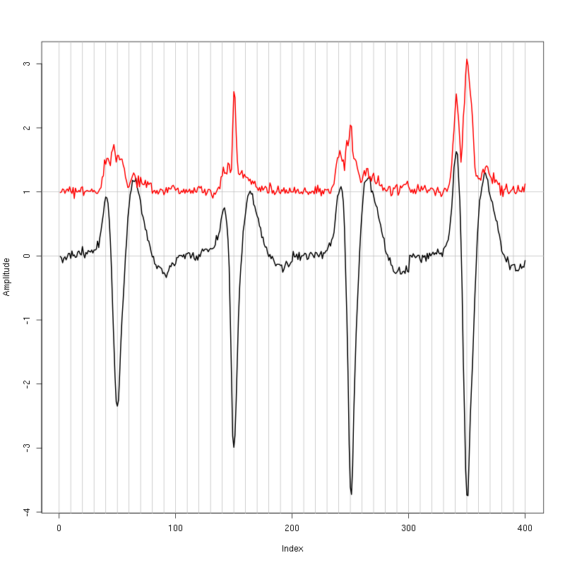
Figure 1: Setting the cut length for the data from tetrode D (channels 10, 12, 14, 15). We see that we need 20 points before the peak and 30 after.

We see that we need roughly 20 points before the peak and 30 after.

2.7 Events

We now cut our events:

evts = mkEvents(sp0,lD,19,30)
summary(evts)

events object deriving from data set: lD.
 Events defined as cuts of 50 sampling points on each of the 4 recording sites.
 The 'reference' time of each event is located at point 20 of the cut.
 There are 760 events in the object.

We can as usual visualize the first 200 events with:

evts[,1:200]

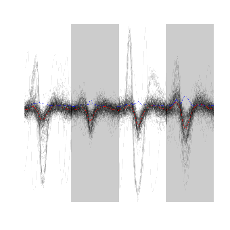
Figure 2: First 200 events for the data from tetrode D (channels 1, 3, 5, 7).

There are superposition and the best way to detect them without excluding good events seems to look for too large negative deviations on both sides of the central valley.

2.8 Removing obvious superposition

We define function goodEvtsFct with:

goodEvtsFct = function(samp,thr=3) {
    samp.med = apply(samp,1,median)
    samp.mad = apply(samp,1,mad)
    under <- samp.med < 0
    samp.r <- apply(samp,2,function(x) {x[under] <- 0;x})
    apply(samp.r,2,function(x) all(x-samp.med > -thr*samp.mad))
}

We apply it with a threshold of 6 times the MAD:

goodEvts = goodEvtsFct(evts,6)

If we look at all the remaining "good" events with (not shown):

evts[,goodEvts]

and at all the "bad" ones (not shown):

evts[,!goodEvts]

we see that our sample cleaning does its job.

2.9 Dimension reduction

We do a PCA on our good events set:

evts.pc = prcomp(t(evts[,goodEvts]))

We look at the projections on the first 4 principle components:

panel.dens = function(x,...) {
  usr = par("usr")
  on.exit(par(usr))
  par(usr = c(usr[1:2], 0, 1.5) )
  d = density(x, adjust=0.5)
  x = d$x
  y = d$y
  y = y/max(y)
  lines(x, y, col="grey50", ...)
}
pairs(evts.pc$x[,1:4],pch=".",gap=0,diag.panel=panel.dens)

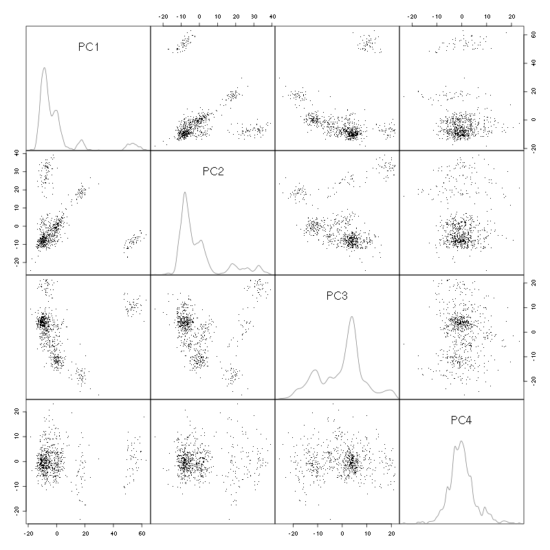
Figure 3: Events from tetrode D (channels 9, 10, 11, 12) projected onto the first 4 PCs.

I see at least 6/7 clusters. We can also look at the projections on the PC pairs defined by the next 4 PCs:

pairs(evts.pc$x[,5:8],pch=".",gap=0,diag.panel=panel.dens)

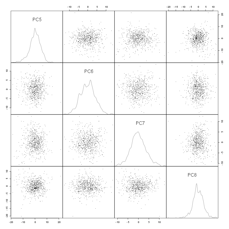
Figure 4: Events from tetrode D (channels 9, 10, 11, 12) projected onto PC 5 to 8.

There is not much structure left beyond the 4th PC.

2.10 Exporting for `GGobi`

We export the events projected onto the first 8 principle components in csv format:

write.csv(evts.pc$x[,1:8],file="tetD_evts.csv")

Using the rotation display of GGobi with the first 3 principle components and the 2D tour with the first 4 components I see 9 clusters. So we will start with a kmeans with 9 centers.

2.11 kmeans clustering with 9

nbc=9
set.seed(20110928,kind="Mersenne-Twister")
km = kmeans(evts.pc$x[,1:4],centers=nbc,iter.max=100,nstart=100)
label = km$cluster
cluster.med = sapply(1:nbc, function(cIdx) median(evts[,goodEvts][,label==cIdx]))
sizeC = sapply(1:nbc,function(cIdx) sum(abs(cluster.med[,cIdx])))
newOrder = sort.int(sizeC,decreasing=TRUE,index.return=TRUE)$ix
cluster.mad = sapply(1:nbc, function(cIdx) {ce = t(evts[,goodEvts]);ce = ce[label==cIdx,];apply(ce,2,mad)})
cluster.med = cluster.med[,newOrder]
cluster.mad = cluster.mad[,newOrder]
labelb = sapply(1:nbc, function(idx) (1:nbc)[newOrder==idx])[label]

We write a new csv file with the data and the labels:

write.csv(cbind(evts.pc$x[,1:5],labelb),file="tetD_sorted.csv")

It gives what was expected.

We get a plot showing the events attributed to each of the first 5 units with:

layout(matrix(1:5,nr=5))
par(mar=c(1,1,1,1))
for (i in (1:5)) plot(evts[,goodEvts][,labelb==i],y.bar=5)

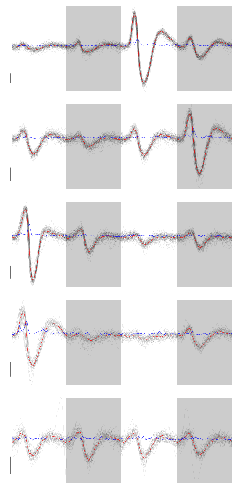
Figure 5: The events of the first five clusters of tetrode D

We get a plot showing the events attributed to each of the last 4 units with:

layout(matrix(1:4,nr=4))
par(mar=c(1,1,1,1))
for (i in (6:9)) plot(evts[,goodEvts][,labelb==i],y.bar=5)

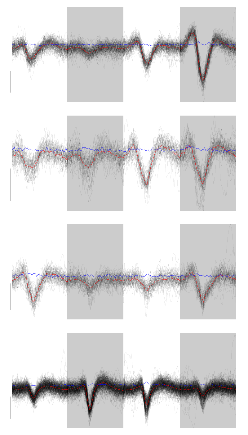
Figure 6: The events of the last four clusters of tetrode D

There are at least two units in cluster 9 but given the events of this clusters have a small amplitude I do not think it is worth going further, we should consider this cluster (as well as the previous 2) as not well isolated.

2.12 Long cuts creation

For the peeling process we need templates that start and end at 0 (we will otherwise generate artifacts when we subtract). We proceed "as usual" with (I tried first with the default value for parameters before and after but I reduced their values after looking at the centers, see the next figure):

c_before = 49
c_after = 80
centers = lapply(1:nbc, function(i)
    mk_center_list(sp0[goodEvts][labelb==i],lD,
                   before=c_before,after=c_after))
names(centers) = paste("Cluster",1:nbc)

We then make sure that our cuts are long enough by looking at them:

layout(matrix(1:nbc,nr=nbc))
par(mar=c(1,4,1,1))
the_range=c(min(sapply(centers,function(l) min(l$center))),
            max(sapply(centers,function(l) max(l$center))))
for (i in 1:nbc) {
    template = centers[[i]]$center
    plot(template,lwd=2,col=2,
         ylim=the_range,type="l",ylab="")
    abline(h=0,col="grey50")
    abline(v=(1:2)*(c_before+c_after)+1,col="grey50")
    lines(filter(template,rep(1,filter_length)/filter_length),
          col=1,lty=3,lwd=2)
    abline(h=-threshold_factor,col="grey",lty=2,lwd=2)
    lines(centers[[i]]$centerD,lwd=2,col=4)
}

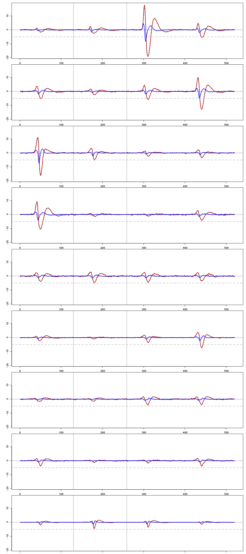
Figure 7: The nine templates (red) together with their first derivative (blue) all with the same scale. The dashed black curve show the templates filtered with the filter used during spike detection and the horizontal dashed grey line shows the detection threshold.

Units 1 to 4 and 6 should be reliably detected, we should miss some events from cluster 5 and many from the last three.

2.13 Peeling

We can now do the peeling.

2.13.1 Round 0

We classify, predict, subtract and check how many non-classified events we get:

round0 = lapply(as.vector(sp0),classify_and_align_evt,
                data=lD,centers=centers,
                before=c_before,after=c_after)
pred0 = predict_data(round0,centers,data_length = dim(lD)[1])
lD_1 = lD - pred0
sum(sapply(round0, function(l) l[[1]] == '?'))

We can see the difference before / after peeling for the data between 1.3 and 1.4 s:

ii = 1:1500 + 1.3*15000
tt = ii/15000
par(mar=c(1,1,1,1))
plot(tt, lD[ii,1], axes = FALSE,
     type="l",ylim=c(-50,10),
     xlab="",ylab="")
lines(tt, lD_1[ii,1], col='red')
lines(tt, lD[ii,2]-15, col='black')
lines(tt, lD_1[ii,2]-15, col='red')
lines(tt, lD[ii,3]-25, col='black')
lines(tt, lD_1[ii,3]-25, col='red')
lines(tt, lD[ii,4]-40, col='black')
lines(tt, lD_1[ii,4]-40, col='red')

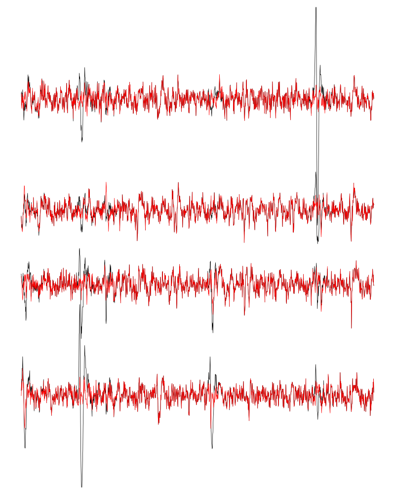
Figure 8: The first peeling illustrated on 100 ms of data, the raw data are in black and the first subtration in red.

2.13.2 Round 1

We keep going, using the subtracted data lD_1 as "raw data", detecting on all sites using the original MAD for normalization:

lDf = -lD_1
lDf = filter(lDf,rep(1,filter_length)/filter_length)
lDf[is.na(lDf)] = 0
lDf = t(t(lDf)/lDf_mad_original)
thrs = threshold_factor*c(1,1,1,1)
bellow.thrs = t(t(lDf) < thrs)
lDfr = lDf
lDfr[bellow.thrs] = 0
remove(lDf)
sp1 = peaks(apply(lDfr,1,sum),15)
remove(lDfr)
sp1

eventsPos object with indexes of 64 events. 
  Mean inter event interval: 4593.48 sampling points, corresponding SD: 6269.96 sampling points 
  Smallest and largest inter event intervals: 18 and 40764 sampling points.

We classify, predict, subtract and check how many non-classified events we get:

round1 = lapply(as.vector(sp1),classify_and_align_evt,
                data=lD_1,centers=centers,
                before=c_before,after=c_after)
pred1 = predict_data(round1,centers,data_length = dim(lD)[1])
lD_2 = lD_1 - pred1
sum(sapply(round1, function(l) l[[1]] == '?'))

We look at what's left with (not shown):

explore(sp1,lD_2,col=c("black","grey50"))

There are 3 large events left so we do one more round.

2.13.3 Round 2

We keep going, using the subtracted data lD_2 as "raw data", detecting on all sites using the original MAD for normalization:

lDf = -lD_2
lDf = filter(lDf,rep(1,filter_length)/filter_length)
lDf[is.na(lDf)] = 0
lDf = t(t(lDf)/lDf_mad_original)
thrs = threshold_factor*c(1,1,1,1)
bellow.thrs = t(t(lDf) < thrs)
lDfr = lDf
lDfr[bellow.thrs] = 0
remove(lDf)
sp2 = peaks(apply(lDfr,1,sum),15)
remove(lDfr)
sp2

eventsPos object with indexes of 16 events. 
  Mean inter event interval: 18151.6 sampling points, corresponding SD: 19193.93 sampling points 
  Smallest and largest inter event intervals: 22 and 73390 sampling points.

We classify, predict, subtract and check how many non-classified events we get:

round2 = lapply(as.vector(sp2),classify_and_align_evt,
                data=lD_2,centers=centers,
                before=c_before,after=c_after)
pred2 = predict_data(round2,centers,data_length = dim(lD)[1])
lD_3 = lD_2 - pred2
sum(sapply(round2, function(l) l[[1]] == '?'))

We look at what's left with (not shown):

explore(sp2,lD_3,col=c("black","grey50"))

There are still 3 large events left so we will do only 2 round in the sequel.

2.14 Getting the spike trains

round_all = c(round0,round1)
spike_trains = lapply(paste("Cluster",1:nbc),
                      function(cn) sort(sapply(round_all[sapply(round_all,
                                                           function(l) l[[1]]==cn)],
                                          function(l) l[[2]]+l[[3]])))
names(spike_trains) = paste("Cluster",1:nbc)

2.15 Getting the inter spike intervals and the forward and backward recurrence times

2.15.1 ISI distributions

We first get the ISI (inter spike intervals) of each unit:

isi = sapply(spike_trains, diff)
names(isi) = names(spike_trains)

We get the ISI ECDF for the five units with:

layout(matrix(1:(nbc+nbc %% 2),nr=ceiling(nbc/2)))
par(mar=c(4,5,6,1))
for (cn in names(isi)) plot_isi(isi[[cn]],main=cn)

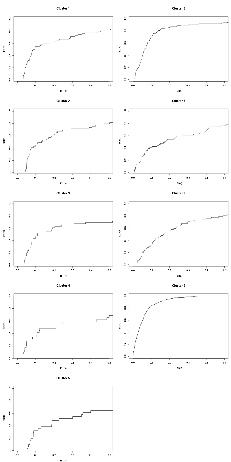
Figure 9: ISI ECDF for the nine units.

2.15.2 Forward and Backward Recurrence Times

The forward recurrence time (FRT) between neuron A and B is the elapsed time between a spike in A and the next spike in B. The backward recurrence time (BRT) is the same thing except that we look for the former spike in B. If A and B are not correlated, the expected density of the FRT is the survival function (1-CDF) of the ISI from B divided by the mean ISI of B (the same holds for the BRT under the null hypothesis after taking the opposite). All that is correct if the data are stationary.

On the data at hand that gives:

layout_matrix = matrix(0,nr=nbc,nc=nbc)
counter = 1
for (i in 1:nbc)
    for (j in 1:nbc)
        if (i != j) {
            layout_matrix[i,j] = counter
            counter = counter +1
        }
layout(layout_matrix)
par(mar=c(4,3,4,1))
for (i in 1:nbc)
    for (j in 1:nbc)
        if (i != j)
            test_rt(spike_trains[[i]],
                    spike_trains[[j]],
                    ylab="",main=paste("Units",i,"and",j))

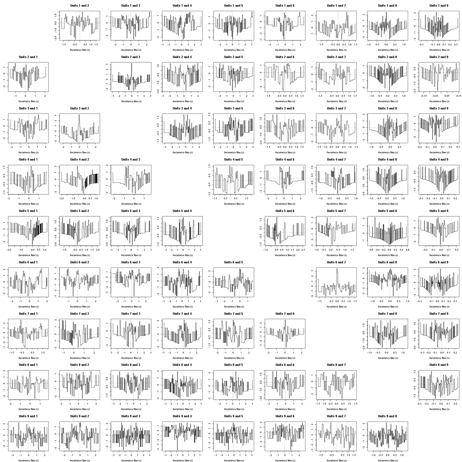
Figure 10: Graphical tests of the Backward and Forward Reccurrence Times distrution agaisnt the null hypothesis (no interaction). If the null is correct, the curves should be IID draws from a standard normal distribution.

2.16 Testing `all_at_once`

We test the function with:

## We need again an un-normalized version of the data
ref_data = get_data(1,"Cis-3-Hexen-1-ol (10^-0) first",
              channels = c("ch10","ch12","ch14","ch15"),
              file="locust20000613.hdf5")
## We can now use our function
aao=all_at_once(data=ref_data, centers, thres=threshold_factor*c(1,1,1,1), 
                filter_length_1=filter_length, filter_length=filter_length, 
                minimalDist_1=15, minimalDist=15, 
                before=c_before, after=c_after, 
                detection_cycle=c(0,0), verbose=2)

The five number summary is:
      ch10           ch12           ch14           ch15     
 Min.   : 818   Min.   : 764   Min.   : 372   Min.   : 128  
 1st Qu.:2005   1st Qu.:1959   1st Qu.:2001   1st Qu.:1984  
 Median :2050   Median :2053   Median :2050   Median :2054  
 Mean   :2048   Mean   :2047   Mean   :2047   Mean   :2050  
 3rd Qu.:2094   3rd Qu.:2145   3rd Qu.:2098   3rd Qu.:2121  
 Max.   :2971   Max.   :2966   Max.   :3581   Max.   :3473  

Doing now round 0 detecting on all sites
    Total Cluster 1 Cluster 2 Cluster 3 Cluster 4 Cluster 5 Cluster 6 Cluster 7 
      760        66        50        47        29        32       123        53 
Cluster 8 Cluster 9         ? 
       62       296         2 

Doing now round 1 detecting on all sites
    Total Cluster 1 Cluster 2 Cluster 3 Cluster 4 Cluster 5 Cluster 6 Cluster 7 
       64         1         0         0         1         0         3         7 
Cluster 8 Cluster 9         ? 
       10        35         7 

Global counts at classification's end:
    Total Cluster 1 Cluster 2 Cluster 3 Cluster 4 Cluster 5 Cluster 6 Cluster 7 
      831        67        50        47        30        32       126        60 
Cluster 8 Cluster 9         ? 
       72       331        16

We see that we are getting back the numbers we obtained before step by step.

We can compare the "old" and "new" centers with (not shown):

layout(matrix(1:nbc,nr=nbc))
par(mar=c(1,4,1,1))
for (i in 1:nbc) {
    plot(centers[[i]]$center,lwd=2,col=2,
         ylim=the_range,type="l")
    abline(h=0,col="grey50")
    abline(v=(c_before+c_after)+1,col="grey50")
    lines(aao$centers[[i]]$center,lwd=1,col=4)
}

They are not exactly identical since the new version is computed with all events (superposed or not) attributed to each neuron.

3 Analyzing a sequence of trials

3.1 Create directories were results get saved

We will carry out an analysis of sequences of many trials with a given odor. At the end of the analysis of the sequence we will save some intermediate R object in a directory we are now creating.:

if (!dir.exists("tetD_analysis"))
    dir.create("tetD_analysis")

We will moreover save the individual spike trains in text format in a directory:

if (!dir.exists("locust20000613_spike_trains"))
    dir.create("locust20000613_spike_trains")

3.2 Define a "taylored" version of `sort_many_trials`

In order to save space and to avoid typos, we define next a taylored version of sort_many_trials:

smt = function(stim_name,
               trial_nbs,
               centers,
               counts) {
    sort_many_trials(inter_trial_time=20*15000,
                     get_data_fct=function(i,s)
                         get_data(i,s,
                                  channels = c("ch10","ch12","ch14","ch15"),
                                  file="locust20000613.hdf5"),
                     stim_name=stim_name,
                     trial_nbs=trial_nbs,
                     centers=centers,
                     counts=counts,
                     all_at_once_call_list=list(thres=threshold_factor*c(1,1,1,1), 
                                                filter_length_1=filter_length, filter_length=filter_length, 
                                                minimalDist_1=15, minimalDist=15, 
                                                before=c_before, after=c_after, 
                                                detection_cycle=c(0,0), verbose=1),
                     layout_matrix=matrix(1:10,nr=5),new_weight_in_update=0.01
                     )
}

4 Systematic analysis of the 50 trials with "pure" `Cis-3-Hexen-1-ol`

4.1 Doing the job

a_Cis_3_Hexen_1_ol_0_f_tetD=smt(stim_name="Cis-3-Hexen-1-ol (10^-0) first",
                                trial_nbs=1:50,
                                centers=aao$centers,
                                counts=aao$counts)

***************
Doing now trial 1 of Cis-3-Hexen-1-ol (10^-0) first
The five number summary is:
      ch10           ch12           ch14           ch15     
 Min.   : 818   Min.   : 764   Min.   : 372   Min.   : 128  
 1st Qu.:2005   1st Qu.:1959   1st Qu.:2001   1st Qu.:1984  
 Median :2050   Median :2053   Median :2050   Median :2054  
 Mean   :2048   Mean   :2047   Mean   :2047   Mean   :2050  
 3rd Qu.:2094   3rd Qu.:2145   3rd Qu.:2098   3rd Qu.:2121  
 Max.   :2971   Max.   :2966   Max.   :3581   Max.   :3473  

Global counts at classification's end:
    Total Cluster 1 Cluster 2 Cluster 3 Cluster 4 Cluster 5 Cluster 6 Cluster 7 
      830        67        50        46        31        33       123        62 
Cluster 8 Cluster 9         ? 
       69       332        17 
Trial 1 done!
******************
***************
Doing now trial 2 of Cis-3-Hexen-1-ol (10^-0) first
The five number summary is:
      ch10           ch12           ch14           ch15     
 Min.   : 669   Min.   : 558   Min.   : 542   Min.   :  21  
 1st Qu.:2005   1st Qu.:1957   1st Qu.:2000   1st Qu.:1984  
 Median :2051   Median :2054   Median :2050   Median :2054  
 Mean   :2048   Mean   :2047   Mean   :2047   Mean   :2050  
 3rd Qu.:2094   3rd Qu.:2148   3rd Qu.:2099   3rd Qu.:2122  
 Max.   :2977   Max.   :2913   Max.   :3634   Max.   :3404  

Global counts at classification's end:
    Total Cluster 1 Cluster 2 Cluster 3 Cluster 4 Cluster 5 Cluster 6 Cluster 7 
      919       108        76        49        13        39       116        63 
Cluster 8 Cluster 9         ? 
       67       370        18 
Trial 2 done!
******************
***************
Doing now trial 3 of Cis-3-Hexen-1-ol (10^-0) first
The five number summary is:
      ch10           ch12           ch14           ch15     
 Min.   : 768   Min.   : 764   Min.   : 450   Min.   : 271  
 1st Qu.:2005   1st Qu.:1957   1st Qu.:2001   1st Qu.:1983  
 Median :2051   Median :2054   Median :2051   Median :2054  
 Mean   :2048   Mean   :2047   Mean   :2047   Mean   :2050  
 3rd Qu.:2095   3rd Qu.:2147   3rd Qu.:2098   3rd Qu.:2122  
 Max.   :3030   Max.   :3046   Max.   :3500   Max.   :3383  

Global counts at classification's end:
    Total Cluster 1 Cluster 2 Cluster 3 Cluster 4 Cluster 5 Cluster 6 Cluster 7 
      944       136       108        44        16        33       112        55 
Cluster 8 Cluster 9         ? 
       78       337        25 
Trial 3 done!
******************
***************
Doing now trial 4 of Cis-3-Hexen-1-ol (10^-0) first
The five number summary is:
      ch10           ch12           ch14           ch15     
 Min.   : 766   Min.   : 811   Min.   : 420   Min.   : 279  
 1st Qu.:2004   1st Qu.:1959   1st Qu.:2002   1st Qu.:1983  
 Median :2051   Median :2053   Median :2051   Median :2054  
 Mean   :2048   Mean   :2047   Mean   :2047   Mean   :2050  
 3rd Qu.:2096   3rd Qu.:2145   3rd Qu.:2097   3rd Qu.:2123  
 Max.   :3047   Max.   :2937   Max.   :3499   Max.   :3342  

Global counts at classification's end:
    Total Cluster 1 Cluster 2 Cluster 3 Cluster 4 Cluster 5 Cluster 6 Cluster 7 
      890        90        90        58        17        31       133        53 
Cluster 8 Cluster 9         ? 
       92       295        31 
Trial 4 done!
******************
***************
Doing now trial 5 of Cis-3-Hexen-1-ol (10^-0) first
The five number summary is:
      ch10           ch12           ch14           ch15     
 Min.   : 714   Min.   : 765   Min.   : 479   Min.   : 244  
 1st Qu.:2004   1st Qu.:1959   1st Qu.:2002   1st Qu.:1983  
 Median :2051   Median :2054   Median :2050   Median :2054  
 Mean   :2048   Mean   :2047   Mean   :2047   Mean   :2050  
 3rd Qu.:2095   3rd Qu.:2144   3rd Qu.:2097   3rd Qu.:2122  
 Max.   :3007   Max.   :2886   Max.   :3413   Max.   :3280  

Global counts at classification's end:
    Total Cluster 1 Cluster 2 Cluster 3 Cluster 4 Cluster 5 Cluster 6 Cluster 7 
      902        98        74        47        14        34       147        59 
Cluster 8 Cluster 9         ? 
       79       325        25 
Trial 5 done!
******************
***************
Doing now trial 6 of Cis-3-Hexen-1-ol (10^-0) first
The five number summary is:
      ch10           ch12           ch14           ch15     
 Min.   : 726   Min.   : 860   Min.   : 493   Min.   : 207  
 1st Qu.:2004   1st Qu.:1958   1st Qu.:2001   1st Qu.:1983  
 Median :2051   Median :2053   Median :2050   Median :2054  
 Mean   :2048   Mean   :2047   Mean   :2047   Mean   :2050  
 3rd Qu.:2095   3rd Qu.:2145   3rd Qu.:2097   3rd Qu.:2122  
 Max.   :3096   Max.   :2961   Max.   :3475   Max.   :3411  

Global counts at classification's end:
    Total Cluster 1 Cluster 2 Cluster 3 Cluster 4 Cluster 5 Cluster 6 Cluster 7 
      871        91        83        53        16        34       116        70 
Cluster 8 Cluster 9         ? 
       85       294        29 
Trial 6 done!
******************
***************
Doing now trial 7 of Cis-3-Hexen-1-ol (10^-0) first
The five number summary is:
      ch10           ch12           ch14           ch15     
 Min.   : 730   Min.   : 911   Min.   : 473   Min.   : 476  
 1st Qu.:2005   1st Qu.:1959   1st Qu.:2002   1st Qu.:1984  
 Median :2051   Median :2053   Median :2051   Median :2054  
 Mean   :2048   Mean   :2047   Mean   :2047   Mean   :2050  
 3rd Qu.:2095   3rd Qu.:2143   3rd Qu.:2096   3rd Qu.:2122  
 Max.   :3021   Max.   :2896   Max.   :3426   Max.   :3340  

Global counts at classification's end:
    Total Cluster 1 Cluster 2 Cluster 3 Cluster 4 Cluster 5 Cluster 6 Cluster 7 
      855        84        66        54        18        29       139        60 
Cluster 8 Cluster 9         ? 
       97       293        15 
Trial 7 done!
******************
***************
Doing now trial 8 of Cis-3-Hexen-1-ol (10^-0) first
The five number summary is:
      ch10           ch12           ch14           ch15     
 Min.   : 661   Min.   : 674   Min.   : 506   Min.   : 490  
 1st Qu.:2004   1st Qu.:1958   1st Qu.:2002   1st Qu.:1983  
 Median :2051   Median :2054   Median :2050   Median :2054  
 Mean   :2048   Mean   :2047   Mean   :2047   Mean   :2050  
 3rd Qu.:2095   3rd Qu.:2146   3rd Qu.:2097   3rd Qu.:2122  
 Max.   :3081   Max.   :2902   Max.   :3515   Max.   :3559  

Global counts at classification's end:
    Total Cluster 1 Cluster 2 Cluster 3 Cluster 4 Cluster 5 Cluster 6 Cluster 7 
      886        92        59        45        12        40       136        69 
Cluster 8 Cluster 9         ? 
       75       325        33 
Trial 8 done!
******************
***************
Doing now trial 9 of Cis-3-Hexen-1-ol (10^-0) first
The five number summary is:
      ch10           ch12           ch14           ch15     
 Min.   : 325   Min.   : 887   Min.   : 448   Min.   :   0  
 1st Qu.:2004   1st Qu.:1958   1st Qu.:2001   1st Qu.:1983  
 Median :2051   Median :2054   Median :2051   Median :2054  
 Mean   :2048   Mean   :2047   Mean   :2047   Mean   :2050  
 3rd Qu.:2096   3rd Qu.:2145   3rd Qu.:2097   3rd Qu.:2122  
 Max.   :3361   Max.   :3085   Max.   :3473   Max.   :3443  

Global counts at classification's end:
    Total Cluster 1 Cluster 2 Cluster 3 Cluster 4 Cluster 5 Cluster 6 Cluster 7 
      881       101        64        59         8        46       123        57 
Cluster 8 Cluster 9         ? 
       77       328        18 
Trial 9 done!
******************
***************
Doing now trial 10 of Cis-3-Hexen-1-ol (10^-0) first
The five number summary is:
      ch10           ch12           ch14           ch15     
 Min.   : 723   Min.   : 813   Min.   : 190   Min.   : 469  
 1st Qu.:2004   1st Qu.:1957   1st Qu.:2001   1st Qu.:1984  
 Median :2051   Median :2054   Median :2051   Median :2054  
 Mean   :2048   Mean   :2047   Mean   :2047   Mean   :2050  
 3rd Qu.:2096   3rd Qu.:2147   3rd Qu.:2097   3rd Qu.:2122  
 Max.   :3071   Max.   :2919   Max.   :3490   Max.   :3414  

Global counts at classification's end:
    Total Cluster 1 Cluster 2 Cluster 3 Cluster 4 Cluster 5 Cluster 6 Cluster 7 
      898        90        83        51        17        42       125        58 
Cluster 8 Cluster 9         ? 
       83       321        28 
Trial 10 done!
******************
***************
Doing now trial 11 of Cis-3-Hexen-1-ol (10^-0) first
The five number summary is:
      ch10           ch12           ch14           ch15     
 Min.   : 323   Min.   : 689   Min.   : 299   Min.   : 273  
 1st Qu.:2004   1st Qu.:1959   1st Qu.:2002   1st Qu.:1984  
 Median :2051   Median :2053   Median :2051   Median :2054  
 Mean   :2048   Mean   :2047   Mean   :2047   Mean   :2050  
 3rd Qu.:2095   3rd Qu.:2145   3rd Qu.:2097   3rd Qu.:2121  
 Max.   :3067   Max.   :2914   Max.   :3564   Max.   :3489  

Global counts at classification's end:
    Total Cluster 1 Cluster 2 Cluster 3 Cluster 4 Cluster 5 Cluster 6 Cluster 7 
      880        77        62        55        11        42       126        54 
Cluster 8 Cluster 9         ? 
       90       345        18 
Trial 11 done!
******************
***************
Doing now trial 12 of Cis-3-Hexen-1-ol (10^-0) first
The five number summary is:
      ch10           ch12           ch14           ch15     
 Min.   : 738   Min.   : 878   Min.   : 356   Min.   : 437  
 1st Qu.:2005   1st Qu.:1958   1st Qu.:2001   1st Qu.:1983  
 Median :2051   Median :2054   Median :2050   Median :2054  
 Mean   :2048   Mean   :2047   Mean   :2047   Mean   :2050  
 3rd Qu.:2095   3rd Qu.:2146   3rd Qu.:2097   3rd Qu.:2122  
 Max.   :3052   Max.   :3205   Max.   :3450   Max.   :3441  

Global counts at classification's end:
    Total Cluster 1 Cluster 2 Cluster 3 Cluster 4 Cluster 5 Cluster 6 Cluster 7 
      897        81        61        62        11        44       132        60 
Cluster 8 Cluster 9         ? 
       84       341        21 
Trial 12 done!
******************
***************
Doing now trial 13 of Cis-3-Hexen-1-ol (10^-0) first
The five number summary is:
      ch10           ch12           ch14           ch15     
 Min.   : 653   Min.   : 833   Min.   : 334   Min.   :  33  
 1st Qu.:2004   1st Qu.:1958   1st Qu.:2002   1st Qu.:1984  
 Median :2051   Median :2054   Median :2050   Median :2054  
 Mean   :2048   Mean   :2047   Mean   :2047   Mean   :2050  
 3rd Qu.:2096   3rd Qu.:2147   3rd Qu.:2097   3rd Qu.:2121  
 Max.   :3088   Max.   :3059   Max.   :3585   Max.   :3383  

Global counts at classification's end:
    Total Cluster 1 Cluster 2 Cluster 3 Cluster 4 Cluster 5 Cluster 6 Cluster 7 
      856        85        82        45        13        45       121        56 
Cluster 8 Cluster 9         ? 
       63       330        16 
Trial 13 done!
******************
***************
Doing now trial 14 of Cis-3-Hexen-1-ol (10^-0) first
The five number summary is:
      ch10           ch12           ch14           ch15     
 Min.   : 621   Min.   : 479   Min.   : 433   Min.   : 249  
 1st Qu.:2004   1st Qu.:1957   1st Qu.:2001   1st Qu.:1983  
 Median :2051   Median :2054   Median :2051   Median :2054  
 Mean   :2048   Mean   :2047   Mean   :2047   Mean   :2050  
 3rd Qu.:2096   3rd Qu.:2147   3rd Qu.:2097   3rd Qu.:2123  
 Max.   :3172   Max.   :3022   Max.   :3536   Max.   :3440  

Global counts at classification's end:
    Total Cluster 1 Cluster 2 Cluster 3 Cluster 4 Cluster 5 Cluster 6 Cluster 7 
      925       100        96        65        11        36       148        57 
Cluster 8 Cluster 9         ? 
       76       316        20 
Trial 14 done!
******************
***************
Doing now trial 15 of Cis-3-Hexen-1-ol (10^-0) first
The five number summary is:
      ch10           ch12           ch14           ch15     
 Min.   : 688   Min.   : 769   Min.   : 412   Min.   : 513  
 1st Qu.:2005   1st Qu.:1958   1st Qu.:2002   1st Qu.:1984  
 Median :2051   Median :2054   Median :2050   Median :2054  
 Mean   :2048   Mean   :2047   Mean   :2047   Mean   :2050  
 3rd Qu.:2095   3rd Qu.:2145   3rd Qu.:2097   3rd Qu.:2121  
 Max.   :3111   Max.   :2912   Max.   :3460   Max.   :3391  

Global counts at classification's end:
    Total Cluster 1 Cluster 2 Cluster 3 Cluster 4 Cluster 5 Cluster 6 Cluster 7 
      866        67        87        46        12        39       123        59 
Cluster 8 Cluster 9         ? 
       91       324        18 
Trial 15 done!
******************
***************
Doing now trial 16 of Cis-3-Hexen-1-ol (10^-0) first
The five number summary is:
      ch10           ch12           ch14           ch15     
 Min.   : 750   Min.   : 797   Min.   : 554   Min.   : 444  
 1st Qu.:2004   1st Qu.:1958   1st Qu.:2002   1st Qu.:1983  
 Median :2051   Median :2054   Median :2050   Median :2053  
 Mean   :2048   Mean   :2047   Mean   :2047   Mean   :2050  
 3rd Qu.:2095   3rd Qu.:2145   3rd Qu.:2097   3rd Qu.:2122  
 Max.   :2989   Max.   :3046   Max.   :3421   Max.   :3431  

Global counts at classification's end:
    Total Cluster 1 Cluster 2 Cluster 3 Cluster 4 Cluster 5 Cluster 6 Cluster 7 
      835        82        49        49        24        40       121        50 
Cluster 8 Cluster 9         ? 
       69       337        14 
Trial 16 done!
******************
***************
Doing now trial 17 of Cis-3-Hexen-1-ol (10^-0) first
The five number summary is:
      ch10           ch12           ch14           ch15     
 Min.   : 656   Min.   : 787   Min.   : 478   Min.   :  75  
 1st Qu.:2005   1st Qu.:1959   1st Qu.:2002   1st Qu.:1983  
 Median :2051   Median :2053   Median :2050   Median :2054  
 Mean   :2048   Mean   :2047   Mean   :2047   Mean   :2050  
 3rd Qu.:2096   3rd Qu.:2145   3rd Qu.:2097   3rd Qu.:2122  
 Max.   :3095   Max.   :3030   Max.   :3420   Max.   :3494  

Global counts at classification's end:
    Total Cluster 1 Cluster 2 Cluster 3 Cluster 4 Cluster 5 Cluster 6 Cluster 7 
      931        79        67        69        16        66       122        60 
Cluster 8 Cluster 9         ? 
       82       340        30 
Trial 17 done!
******************
***************
Doing now trial 18 of Cis-3-Hexen-1-ol (10^-0) first
The five number summary is:
      ch10           ch12           ch14           ch15     
 Min.   : 680   Min.   : 693   Min.   : 376   Min.   :   0  
 1st Qu.:2005   1st Qu.:1959   1st Qu.:2002   1st Qu.:1984  
 Median :2051   Median :2053   Median :2051   Median :2053  
 Mean   :2048   Mean   :2047   Mean   :2047   Mean   :2050  
 3rd Qu.:2095   3rd Qu.:2145   3rd Qu.:2097   3rd Qu.:2121  
 Max.   :3008   Max.   :2962   Max.   :3402   Max.   :3707  

Global counts at classification's end:
    Total Cluster 1 Cluster 2 Cluster 3 Cluster 4 Cluster 5 Cluster 6 Cluster 7 
      864        95        54        63         4        46       132        49 
Cluster 8 Cluster 9         ? 
       81       327        13 
Trial 18 done!
******************
***************
Doing now trial 19 of Cis-3-Hexen-1-ol (10^-0) first
The five number summary is:
      ch10           ch12           ch14           ch15     
 Min.   : 678   Min.   : 887   Min.   : 543   Min.   : 483  
 1st Qu.:2004   1st Qu.:1958   1st Qu.:2002   1st Qu.:1983  
 Median :2051   Median :2053   Median :2051   Median :2054  
 Mean   :2048   Mean   :2047   Mean   :2047   Mean   :2050  
 3rd Qu.:2095   3rd Qu.:2146   3rd Qu.:2097   3rd Qu.:2122  
 Max.   :2987   Max.   :2937   Max.   :3364   Max.   :3339  

Global counts at classification's end:
    Total Cluster 1 Cluster 2 Cluster 3 Cluster 4 Cluster 5 Cluster 6 Cluster 7 
      948        86        84        53        21        45       117        64 
Cluster 8 Cluster 9         ? 
       74       386        18 
Trial 19 done!
******************
***************
Doing now trial 20 of Cis-3-Hexen-1-ol (10^-0) first
The five number summary is:
      ch10           ch12           ch14           ch15     
 Min.   : 701   Min.   : 934   Min.   : 353   Min.   : 471  
 1st Qu.:2004   1st Qu.:1959   1st Qu.:2002   1st Qu.:1984  
 Median :2051   Median :2053   Median :2050   Median :2054  
 Mean   :2048   Mean   :2047   Mean   :2047   Mean   :2050  
 3rd Qu.:2095   3rd Qu.:2144   3rd Qu.:2096   3rd Qu.:2121  
 Max.   :3077   Max.   :3035   Max.   :3414   Max.   :3384  

Global counts at classification's end:
    Total Cluster 1 Cluster 2 Cluster 3 Cluster 4 Cluster 5 Cluster 6 Cluster 7 
      857        75        54        69        10        42       131        46 
Cluster 8 Cluster 9         ? 
       86       329        15 
Trial 20 done!
******************
***************
Doing now trial 21 of Cis-3-Hexen-1-ol (10^-0) first
The five number summary is:
      ch10           ch12           ch14           ch15     
 Min.   : 741   Min.   : 619   Min.   : 529   Min.   : 350  
 1st Qu.:2005   1st Qu.:1958   1st Qu.:2001   1st Qu.:1983  
 Median :2051   Median :2054   Median :2051   Median :2054  
 Mean   :2048   Mean   :2047   Mean   :2047   Mean   :2050  
 3rd Qu.:2095   3rd Qu.:2146   3rd Qu.:2098   3rd Qu.:2123  
 Max.   :3042   Max.   :3026   Max.   :3346   Max.   :3475  

Global counts at classification's end:
    Total Cluster 1 Cluster 2 Cluster 3 Cluster 4 Cluster 5 Cluster 6 Cluster 7 
      921       104        60        66         8        37       148        40 
Cluster 8 Cluster 9         ? 
       89       343        26 
Trial 21 done!
******************
***************
Doing now trial 22 of Cis-3-Hexen-1-ol (10^-0) first
The five number summary is:
      ch10           ch12           ch14           ch15     
 Min.   : 678   Min.   : 869   Min.   : 521   Min.   :  51  
 1st Qu.:2004   1st Qu.:1957   1st Qu.:2001   1st Qu.:1983  
 Median :2051   Median :2053   Median :2051   Median :2054  
 Mean   :2048   Mean   :2047   Mean   :2047   Mean   :2050  
 3rd Qu.:2095   3rd Qu.:2147   3rd Qu.:2098   3rd Qu.:2122  
 Max.   :3030   Max.   :3017   Max.   :3414   Max.   :3454  

Global counts at classification's end:
    Total Cluster 1 Cluster 2 Cluster 3 Cluster 4 Cluster 5 Cluster 6 Cluster 7 
      887        97       120        38        16        36       103        53 
Cluster 8 Cluster 9         ? 
       86       317        21 
Trial 22 done!
******************
***************
Doing now trial 23 of Cis-3-Hexen-1-ol (10^-0) first
The five number summary is:
      ch10           ch12           ch14           ch15     
 Min.   : 627   Min.   : 809   Min.   : 506   Min.   :   0  
 1st Qu.:2005   1st Qu.:1958   1st Qu.:2002   1st Qu.:1983  
 Median :2051   Median :2053   Median :2050   Median :2054  
 Mean   :2048   Mean   :2047   Mean   :2047   Mean   :2050  
 3rd Qu.:2095   3rd Qu.:2144   3rd Qu.:2096   3rd Qu.:2122  
 Max.   :3033   Max.   :2963   Max.   :3395   Max.   :3420  

Global counts at classification's end:
    Total Cluster 1 Cluster 2 Cluster 3 Cluster 4 Cluster 5 Cluster 6 Cluster 7 
      828        97        68        62        13        36       128        45 
Cluster 8 Cluster 9         ? 
       75       293        11 
Trial 23 done!
******************
***************
Doing now trial 24 of Cis-3-Hexen-1-ol (10^-0) first
The five number summary is:
      ch10           ch12           ch14           ch15     
 Min.   : 622   Min.   : 822   Min.   : 602   Min.   : 322  
 1st Qu.:2005   1st Qu.:1959   1st Qu.:2003   1st Qu.:1984  
 Median :2051   Median :2053   Median :2050   Median :2054  
 Mean   :2048   Mean   :2047   Mean   :2047   Mean   :2050  
 3rd Qu.:2095   3rd Qu.:2144   3rd Qu.:2096   3rd Qu.:2122  
 Max.   :3074   Max.   :3018   Max.   :3369   Max.   :3362  

Global counts at classification's end:
    Total Cluster 1 Cluster 2 Cluster 3 Cluster 4 Cluster 5 Cluster 6 Cluster 7 
      884        79        76        71        10        44       123        49 
Cluster 8 Cluster 9         ? 
       92       327        13 
Trial 24 done!
******************
***************
Doing now trial 25 of Cis-3-Hexen-1-ol (10^-0) first
The five number summary is:
      ch10           ch12           ch14           ch15     
 Min.   : 670   Min.   : 690   Min.   : 621   Min.   : 369  
 1st Qu.:2004   1st Qu.:1958   1st Qu.:2002   1st Qu.:1983  
 Median :2051   Median :2054   Median :2051   Median :2054  
 Mean   :2048   Mean   :2047   Mean   :2047   Mean   :2050  
 3rd Qu.:2095   3rd Qu.:2146   3rd Qu.:2097   3rd Qu.:2122  
 Max.   :3016   Max.   :3039   Max.   :3299   Max.   :3315  

Global counts at classification's end:
    Total Cluster 1 Cluster 2 Cluster 3 Cluster 4 Cluster 5 Cluster 6 Cluster 7 
      890        79       103        62        20        57       121        46 
Cluster 8 Cluster 9         ? 
       55       324        23 
Trial 25 done!
******************
***************
Doing now trial 26 of Cis-3-Hexen-1-ol (10^-0) first
The five number summary is:
      ch10           ch12           ch14           ch15     
 Min.   : 508   Min.   : 860   Min.   : 700   Min.   : 396  
 1st Qu.:2006   1st Qu.:1961   1st Qu.:2003   1st Qu.:1985  
 Median :2051   Median :2053   Median :2050   Median :2053  
 Mean   :2048   Mean   :2047   Mean   :2047   Mean   :2050  
 3rd Qu.:2094   3rd Qu.:2142   3rd Qu.:2095   3rd Qu.:2120  
 Max.   :3076   Max.   :2857   Max.   :3268   Max.   :3280  

Global counts at classification's end:
    Total Cluster 1 Cluster 2 Cluster 3 Cluster 4 Cluster 5 Cluster 6 Cluster 7 
      808        76        50        48        10        39       100        53 
Cluster 8 Cluster 9         ? 
      102       315        15 
Trial 26 done!
******************
***************
Doing now trial 27 of Cis-3-Hexen-1-ol (10^-0) first
The five number summary is:
      ch10           ch12           ch14           ch15     
 Min.   : 594   Min.   : 951   Min.   : 532   Min.   : 546  
 1st Qu.:2005   1st Qu.:1960   1st Qu.:2003   1st Qu.:1985  
 Median :2051   Median :2053   Median :2050   Median :2054  
 Mean   :2048   Mean   :2047   Mean   :2047   Mean   :2050  
 3rd Qu.:2094   3rd Qu.:2143   3rd Qu.:2095   3rd Qu.:2120  
 Max.   :2931   Max.   :2937   Max.   :3281   Max.   :3221  

Global counts at classification's end:
    Total Cluster 1 Cluster 2 Cluster 3 Cluster 4 Cluster 5 Cluster 6 Cluster 7 
      778        84        48        60        12        32       124        41 
Cluster 8 Cluster 9         ? 
       75       285        17 
Trial 27 done!
******************
***************
Doing now trial 28 of Cis-3-Hexen-1-ol (10^-0) first
The five number summary is:
      ch10           ch12           ch14           ch15     
 Min.   : 708   Min.   : 645   Min.   : 652   Min.   : 528  
 1st Qu.:2005   1st Qu.:1960   1st Qu.:2003   1st Qu.:1985  
 Median :2051   Median :2053   Median :2050   Median :2054  
 Mean   :2048   Mean   :2047   Mean   :2047   Mean   :2050  
 3rd Qu.:2094   3rd Qu.:2143   3rd Qu.:2095   3rd Qu.:2121  
 Max.   :2945   Max.   :2923   Max.   :3188   Max.   :3201  

Global counts at classification's end:
    Total Cluster 1 Cluster 2 Cluster 3 Cluster 4 Cluster 5 Cluster 6 Cluster 7 
      812        91        58        47         8        43       121        51 
Cluster 8 Cluster 9         ? 
       88       286        19 
Trial 28 done!
******************
***************
Doing now trial 29 of Cis-3-Hexen-1-ol (10^-0) first
The five number summary is:
      ch10           ch12           ch14           ch15     
 Min.   : 761   Min.   : 750   Min.   : 612   Min.   : 430  
 1st Qu.:2005   1st Qu.:1959   1st Qu.:2003   1st Qu.:1985  
 Median :2051   Median :2054   Median :2050   Median :2053  
 Mean   :2048   Mean   :2047   Mean   :2047   Mean   :2050  
 3rd Qu.:2094   3rd Qu.:2144   3rd Qu.:2096   3rd Qu.:2121  
 Max.   :2848   Max.   :2924   Max.   :3145   Max.   :3188  

Global counts at classification's end:
    Total Cluster 1 Cluster 2 Cluster 3 Cluster 4 Cluster 5 Cluster 6 Cluster 7 
      876        75        69        56        16        43       115        41 
Cluster 8 Cluster 9         ? 
      105       333        23 
Trial 29 done!
******************
***************
Doing now trial 30 of Cis-3-Hexen-1-ol (10^-0) first
The five number summary is:
      ch10           ch12           ch14           ch15     
 Min.   : 836   Min.   : 970   Min.   : 660   Min.   : 537  
 1st Qu.:2006   1st Qu.:1961   1st Qu.:2003   1st Qu.:1985  
 Median :2051   Median :2053   Median :2050   Median :2053  
 Mean   :2048   Mean   :2047   Mean   :2047   Mean   :2050  
 3rd Qu.:2094   3rd Qu.:2142   3rd Qu.:2095   3rd Qu.:2119  
 Max.   :2867   Max.   :2817   Max.   :3195   Max.   :3241  

Global counts at classification's end:
    Total Cluster 1 Cluster 2 Cluster 3 Cluster 4 Cluster 5 Cluster 6 Cluster 7 
      759        62        40        61        22        50        96        30 
Cluster 8 Cluster 9         ? 
       89       297        12 
Trial 30 done!
******************
***************
Doing now trial 31 of Cis-3-Hexen-1-ol (10^-0) first
The five number summary is:
      ch10           ch12           ch14           ch15     
 Min.   : 872   Min.   : 697   Min.   : 737   Min.   : 660  
 1st Qu.:2005   1st Qu.:1959   1st Qu.:2003   1st Qu.:1984  
 Median :2051   Median :2053   Median :2051   Median :2054  
 Mean   :2048   Mean   :2047   Mean   :2047   Mean   :2050  
 3rd Qu.:2094   3rd Qu.:2144   3rd Qu.:2096   3rd Qu.:2120  
 Max.   :2946   Max.   :2879   Max.   :3298   Max.   :3243  

Global counts at classification's end:
    Total Cluster 1 Cluster 2 Cluster 3 Cluster 4 Cluster 5 Cluster 6 Cluster 7 
      850        80        68        46        20        41       107        62 
Cluster 8 Cluster 9         ? 
       77       327        22 
Trial 31 done!
******************
***************
Doing now trial 32 of Cis-3-Hexen-1-ol (10^-0) first
The five number summary is:
      ch10           ch12           ch14           ch15     
 Min.   : 709   Min.   : 733   Min.   : 588   Min.   : 589  
 1st Qu.:2005   1st Qu.:1959   1st Qu.:2003   1st Qu.:1985  
 Median :2051   Median :2053   Median :2050   Median :2054  
 Mean   :2048   Mean   :2047   Mean   :2047   Mean   :2050  
 3rd Qu.:2095   3rd Qu.:2144   3rd Qu.:2096   3rd Qu.:2121  
 Max.   :2904   Max.   :3012   Max.   :3241   Max.   :3170  

Global counts at classification's end:
    Total Cluster 1 Cluster 2 Cluster 3 Cluster 4 Cluster 5 Cluster 6 Cluster 7 
      861        77        86        62        10        41       110        45 
Cluster 8 Cluster 9         ? 
       92       316        22 
Trial 32 done!
******************
***************
Doing now trial 33 of Cis-3-Hexen-1-ol (10^-0) first
The five number summary is:
      ch10           ch12           ch14           ch15     
 Min.   : 605   Min.   : 862   Min.   : 562   Min.   : 360  
 1st Qu.:2006   1st Qu.:1959   1st Qu.:2003   1st Qu.:1985  
 Median :2051   Median :2053   Median :2050   Median :2054  
 Mean   :2048   Mean   :2047   Mean   :2047   Mean   :2050  
 3rd Qu.:2094   3rd Qu.:2143   3rd Qu.:2095   3rd Qu.:2120  
 Max.   :3062   Max.   :2939   Max.   :3270   Max.   :3329  

Global counts at classification's end:
    Total Cluster 1 Cluster 2 Cluster 3 Cluster 4 Cluster 5 Cluster 6 Cluster 7 
      831        94        62        61        16        37       125        51 
Cluster 8 Cluster 9         ? 
       77       293        15 
Trial 33 done!
******************
***************
Doing now trial 34 of Cis-3-Hexen-1-ol (10^-0) first
The five number summary is:
      ch10           ch12           ch14           ch15     
 Min.   : 796   Min.   : 716   Min.   : 683   Min.   : 168  
 1st Qu.:2006   1st Qu.:1959   1st Qu.:2002   1st Qu.:1985  
 Median :2051   Median :2053   Median :2051   Median :2054  
 Mean   :2048   Mean   :2047   Mean   :2047   Mean   :2050  
 3rd Qu.:2094   3rd Qu.:2144   3rd Qu.:2096   3rd Qu.:2120  
 Max.   :2909   Max.   :3084   Max.   :3266   Max.   :3277  

Global counts at classification's end:
    Total Cluster 1 Cluster 2 Cluster 3 Cluster 4 Cluster 5 Cluster 6 Cluster 7 
      844        79        61        78        12        32       126        46 
Cluster 8 Cluster 9         ? 
       94       304        12 
Trial 34 done!
******************
***************
Doing now trial 35 of Cis-3-Hexen-1-ol (10^-0) first
The five number summary is:
      ch10           ch12           ch14           ch15     
 Min.   : 860   Min.   : 814   Min.   : 647   Min.   : 614  
 1st Qu.:2006   1st Qu.:1959   1st Qu.:2003   1st Qu.:1985  
 Median :2051   Median :2053   Median :2050   Median :2054  
 Mean   :2048   Mean   :2047   Mean   :2047   Mean   :2050  
 3rd Qu.:2094   3rd Qu.:2144   3rd Qu.:2096   3rd Qu.:2120  
 Max.   :2909   Max.   :2908   Max.   :3227   Max.   :3413  

Global counts at classification's end:
    Total Cluster 1 Cluster 2 Cluster 3 Cluster 4 Cluster 5 Cluster 6 Cluster 7 
      827        95        42        64        11        44       118        46 
Cluster 8 Cluster 9         ? 
       68       328        11 
Trial 35 done!
******************
***************
Doing now trial 36 of Cis-3-Hexen-1-ol (10^-0) first
The five number summary is:
      ch10           ch12           ch14           ch15     
 Min.   : 844   Min.   : 794   Min.   : 686   Min.   : 428  
 1st Qu.:2005   1st Qu.:1958   1st Qu.:2002   1st Qu.:1985  
 Median :2051   Median :2054   Median :2050   Median :2054  
 Mean   :2048   Mean   :2047   Mean   :2047   Mean   :2050  
 3rd Qu.:2095   3rd Qu.:2145   3rd Qu.:2096   3rd Qu.:2120  
 Max.   :2957   Max.   :2998   Max.   :3227   Max.   :3213  

Global counts at classification's end:
    Total Cluster 1 Cluster 2 Cluster 3 Cluster 4 Cluster 5 Cluster 6 Cluster 7 
      889        95       105        39        11        38       116        50 
Cluster 8 Cluster 9         ? 
       74       341        20 
Trial 36 done!
******************
***************
Doing now trial 37 of Cis-3-Hexen-1-ol (10^-0) first
The five number summary is:
      ch10           ch12           ch14           ch15     
 Min.   : 803   Min.   : 667   Min.   : 708   Min.   : 660  
 1st Qu.:2005   1st Qu.:1958   1st Qu.:2003   1st Qu.:1985  
 Median :2051   Median :2053   Median :2050   Median :2053  
 Mean   :2048   Mean   :2047   Mean   :2047   Mean   :2050  
 3rd Qu.:2094   3rd Qu.:2144   3rd Qu.:2096   3rd Qu.:2120  
 Max.   :2896   Max.   :2922   Max.   :3222   Max.   :3240  

Global counts at classification's end:
    Total Cluster 1 Cluster 2 Cluster 3 Cluster 4 Cluster 5 Cluster 6 Cluster 7 
      833        89        88        49         9        32       103        46 
Cluster 8 Cluster 9         ? 
       67       324        26 
Trial 37 done!
******************
***************
Doing now trial 38 of Cis-3-Hexen-1-ol (10^-0) first
The five number summary is:
      ch10           ch12           ch14           ch15     
 Min.   : 861   Min.   : 817   Min.   : 711   Min.   : 173  
 1st Qu.:2006   1st Qu.:1961   1st Qu.:2003   1st Qu.:1985  
 Median :2051   Median :2053   Median :2050   Median :2053  
 Mean   :2048   Mean   :2047   Mean   :2047   Mean   :2050  
 3rd Qu.:2094   3rd Qu.:2141   3rd Qu.:2094   3rd Qu.:2119  
 Max.   :2949   Max.   :2900   Max.   :3285   Max.   :3421  

Global counts at classification's end:
    Total Cluster 1 Cluster 2 Cluster 3 Cluster 4 Cluster 5 Cluster 6 Cluster 7 
      773        74        65        52        13        41       103        42 
Cluster 8 Cluster 9         ? 
       65       302        16 
Trial 38 done!
******************
***************
Doing now trial 39 of Cis-3-Hexen-1-ol (10^-0) first
The five number summary is:
      ch10           ch12           ch14           ch15     
 Min.   : 490   Min.   : 781   Min.   : 589   Min.   : 459  
 1st Qu.:2005   1st Qu.:1959   1st Qu.:2002   1st Qu.:1985  
 Median :2051   Median :2053   Median :2051   Median :2054  
 Mean   :2048   Mean   :2047   Mean   :2047   Mean   :2050  
 3rd Qu.:2095   3rd Qu.:2144   3rd Qu.:2096   3rd Qu.:2121  
 Max.   :3279   Max.   :2887   Max.   :3291   Max.   :3275  

Global counts at classification's end:
    Total Cluster 1 Cluster 2 Cluster 3 Cluster 4 Cluster 5 Cluster 6 Cluster 7 
      855        81        79        75        16        47       117        44 
Cluster 8 Cluster 9         ? 
       68       315        13 
Trial 39 done!
******************
***************
Doing now trial 40 of Cis-3-Hexen-1-ol (10^-0) first
The five number summary is:
      ch10           ch12           ch14           ch15     
 Min.   : 783   Min.   : 636   Min.   : 466   Min.   : 626  
 1st Qu.:2005   1st Qu.:1960   1st Qu.:2003   1st Qu.:1985  
 Median :2051   Median :2053   Median :2050   Median :2053  
 Mean   :2048   Mean   :2047   Mean   :2047   Mean   :2050  
 3rd Qu.:2094   3rd Qu.:2143   3rd Qu.:2095   3rd Qu.:2120  
 Max.   :2932   Max.   :3022   Max.   :3299   Max.   :3315  

Global counts at classification's end:
    Total Cluster 1 Cluster 2 Cluster 3 Cluster 4 Cluster 5 Cluster 6 Cluster 7 
      768        73        54        60        17        49        87        43 
Cluster 8 Cluster 9         ? 
       84       289        12 
Trial 40 done!
******************
***************
Doing now trial 41 of Cis-3-Hexen-1-ol (10^-0) first
The five number summary is:
      ch10           ch12           ch14           ch15     
 Min.   : 598   Min.   : 747   Min.   : 645   Min.   : 370  
 1st Qu.:2005   1st Qu.:1959   1st Qu.:2002   1st Qu.:1985  
 Median :2051   Median :2053   Median :2051   Median :2054  
 Mean   :2048   Mean   :2047   Mean   :2047   Mean   :2050  
 3rd Qu.:2095   3rd Qu.:2144   3rd Qu.:2096   3rd Qu.:2121  
 Max.   :3128   Max.   :3347   Max.   :3437   Max.   :3449  

Global counts at classification's end:
    Total Cluster 1 Cluster 2 Cluster 3 Cluster 4 Cluster 5 Cluster 6 Cluster 7 
      853        80        85        72        17        56        91        51 
Cluster 8 Cluster 9         ? 
       99       288        14 
Trial 41 done!
******************
***************
Doing now trial 42 of Cis-3-Hexen-1-ol (10^-0) first
The five number summary is:
      ch10           ch12           ch14           ch15     
 Min.   : 814   Min.   : 911   Min.   : 695   Min.   : 498  
 1st Qu.:2005   1st Qu.:1960   1st Qu.:2002   1st Qu.:1984  
 Median :2051   Median :2053   Median :2050   Median :2054  
 Mean   :2048   Mean   :2047   Mean   :2047   Mean   :2050  
 3rd Qu.:2094   3rd Qu.:2142   3rd Qu.:2096   3rd Qu.:2120  
 Max.   :2983   Max.   :2925   Max.   :3292   Max.   :3358  

Global counts at classification's end:
    Total Cluster 1 Cluster 2 Cluster 3 Cluster 4 Cluster 5 Cluster 6 Cluster 7 
      748        85        80        55        10        43        87        53 
Cluster 8 Cluster 9         ? 
       57       263        15 
Trial 42 done!
******************
***************
Doing now trial 43 of Cis-3-Hexen-1-ol (10^-0) first
The five number summary is:
      ch10           ch12           ch14           ch15     
 Min.   : 682   Min.   : 682   Min.   : 574   Min.   : 327  
 1st Qu.:2005   1st Qu.:1960   1st Qu.:2003   1st Qu.:1985  
 Median :2051   Median :2053   Median :2050   Median :2053  
 Mean   :2048   Mean   :2047   Mean   :2047   Mean   :2050  
 3rd Qu.:2094   3rd Qu.:2142   3rd Qu.:2096   3rd Qu.:2120  
 Max.   :2920   Max.   :2872   Max.   :3352   Max.   :3290  

Global counts at classification's end:
    Total Cluster 1 Cluster 2 Cluster 3 Cluster 4 Cluster 5 Cluster 6 Cluster 7 
      831        91        69        61        14        44        92        42 
Cluster 8 Cluster 9         ? 
       89       313        16 
Trial 43 done!
******************
***************
Doing now trial 44 of Cis-3-Hexen-1-ol (10^-0) first
The five number summary is:
      ch10           ch12           ch14           ch15     
 Min.   : 812   Min.   : 771   Min.   : 650   Min.   : 485  
 1st Qu.:2005   1st Qu.:1960   1st Qu.:2002   1st Qu.:1984  
 Median :2051   Median :2053   Median :2050   Median :2054  
 Mean   :2048   Mean   :2047   Mean   :2047   Mean   :2050  
 3rd Qu.:2095   3rd Qu.:2144   3rd Qu.:2096   3rd Qu.:2121  
 Max.   :3012   Max.   :3095   Max.   :3261   Max.   :3318  

Global counts at classification's end:
    Total Cluster 1 Cluster 2 Cluster 3 Cluster 4 Cluster 5 Cluster 6 Cluster 7 
      874        92        68        61        13        52       117        64 
Cluster 8 Cluster 9         ? 
       76       308        23 
Trial 44 done!
******************
***************
Doing now trial 45 of Cis-3-Hexen-1-ol (10^-0) first
The five number summary is:
      ch10           ch12           ch14           ch15     
 Min.   : 799   Min.   : 799   Min.   : 613   Min.   : 370  
 1st Qu.:2005   1st Qu.:1959   1st Qu.:2002   1st Qu.:1984  
 Median :2051   Median :2053   Median :2051   Median :2054  
 Mean   :2048   Mean   :2047   Mean   :2047   Mean   :2050  
 3rd Qu.:2095   3rd Qu.:2144   3rd Qu.:2097   3rd Qu.:2121  
 Max.   :2928   Max.   :2882   Max.   :3324   Max.   :3363  

Global counts at classification's end:
    Total Cluster 1 Cluster 2 Cluster 3 Cluster 4 Cluster 5 Cluster 6 Cluster 7 
      887       104       102        53         8        55        91        55 
Cluster 8 Cluster 9         ? 
       83       319        17 
Trial 45 done!
******************
***************
Doing now trial 46 of Cis-3-Hexen-1-ol (10^-0) first
The five number summary is:
      ch10           ch12           ch14           ch15     
 Min.   : 732   Min.   : 711   Min.   : 621   Min.   :  78  
 1st Qu.:2005   1st Qu.:1960   1st Qu.:2003   1st Qu.:1984  
 Median :2051   Median :2053   Median :2050   Median :2054  
 Mean   :2048   Mean   :2047   Mean   :2047   Mean   :2050  
 3rd Qu.:2095   3rd Qu.:2143   3rd Qu.:2096   3rd Qu.:2120  
 Max.   :2961   Max.   :2834   Max.   :3347   Max.   :3595  

Global counts at classification's end:
    Total Cluster 1 Cluster 2 Cluster 3 Cluster 4 Cluster 5 Cluster 6 Cluster 7 
      822        71        83        49        12        57        90        64 
Cluster 8 Cluster 9         ? 
       87       290        19 
Trial 46 done!
******************
***************
Doing now trial 47 of Cis-3-Hexen-1-ol (10^-0) first
The five number summary is:
      ch10           ch12           ch14           ch15     
 Min.   : 754   Min.   : 355   Min.   : 570   Min.   : 319  
 1st Qu.:2006   1st Qu.:1961   1st Qu.:2003   1st Qu.:1985  
 Median :2051   Median :2053   Median :2050   Median :2054  
 Mean   :2048   Mean   :2047   Mean   :2047   Mean   :2050  
 3rd Qu.:2094   3rd Qu.:2142   3rd Qu.:2095   3rd Qu.:2120  
 Max.   :3029   Max.   :3072   Max.   :3339   Max.   :3397  

Global counts at classification's end:
    Total Cluster 1 Cluster 2 Cluster 3 Cluster 4 Cluster 5 Cluster 6 Cluster 7 
      800        77        59        57        13        35        93        42 
Cluster 8 Cluster 9         ? 
       79       329        16 
Trial 47 done!
******************
***************
Doing now trial 48 of Cis-3-Hexen-1-ol (10^-0) first
The five number summary is:
      ch10           ch12           ch14           ch15     
 Min.   : 676   Min.   : 752   Min.   : 612   Min.   : 407  
 1st Qu.:2005   1st Qu.:1960   1st Qu.:2002   1st Qu.:1985  
 Median :2051   Median :2053   Median :2050   Median :2053  
 Mean   :2048   Mean   :2047   Mean   :2047   Mean   :2050  
 3rd Qu.:2095   3rd Qu.:2142   3rd Qu.:2095   3rd Qu.:2120  
 Max.   :2986   Max.   :2880   Max.   :3335   Max.   :3498  

Global counts at classification's end:
    Total Cluster 1 Cluster 2 Cluster 3 Cluster 4 Cluster 5 Cluster 6 Cluster 7 
      794        88        62        44        15        44       107        40 
Cluster 8 Cluster 9         ? 
       76       304        14 
Trial 48 done!
******************
***************
Doing now trial 49 of Cis-3-Hexen-1-ol (10^-0) first
The five number summary is:
      ch10           ch12           ch14           ch15     
 Min.   : 755   Min.   : 715   Min.   : 608   Min.   : 243  
 1st Qu.:2004   1st Qu.:1958   1st Qu.:2002   1st Qu.:1984  
 Median :2051   Median :2053   Median :2051   Median :2054  
 Mean   :2048   Mean   :2047   Mean   :2047   Mean   :2050  
 3rd Qu.:2095   3rd Qu.:2145   3rd Qu.:2097   3rd Qu.:2121  
 Max.   :2996   Max.   :2928   Max.   :3258   Max.   :3478  

Global counts at classification's end:
    Total Cluster 1 Cluster 2 Cluster 3 Cluster 4 Cluster 5 Cluster 6 Cluster 7 
      920       114       140        41        16        40        93        39 
Cluster 8 Cluster 9         ? 
       77       335        25 
Trial 49 done!
******************
***************
Doing now trial 50 of Cis-3-Hexen-1-ol (10^-0) first
The five number summary is:
      ch10           ch12           ch14           ch15     
 Min.   : 799   Min.   : 732   Min.   : 594   Min.   : 178  
 1st Qu.:2005   1st Qu.:1961   1st Qu.:2003   1st Qu.:1985  
 Median :2051   Median :2053   Median :2050   Median :2053  
 Mean   :2048   Mean   :2047   Mean   :2047   Mean   :2050  
 3rd Qu.:2094   3rd Qu.:2141   3rd Qu.:2095   3rd Qu.:2119  
 Max.   :2986   Max.   :2844   Max.   :3250   Max.   :3386  

Global counts at classification's end:
    Total Cluster 1 Cluster 2 Cluster 3 Cluster 4 Cluster 5 Cluster 6 Cluster 7 
      766        61        68        49         8        32        92        54 
Cluster 8 Cluster 9         ? 
       75       309        18 
Trial 50 done!
******************

4.2 Diagnostic plots

The counts evolution is:

counts_evolution(a_Cis_3_Hexen_1_ol_0_f_tetD)

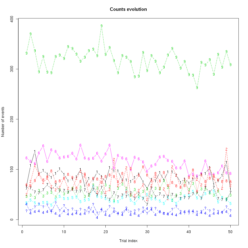
Figure 11: Evolution of the number of events attributed to each unit (1 to 9) or unclassified ("?") during the 50 trials with "pure" Cis_3_Hexen_1_ol for tetrode D.

The waveform evolution is:

waveform_evolution(a_Cis_3_Hexen_1_ol_0_f_tetD,threshold_factor)

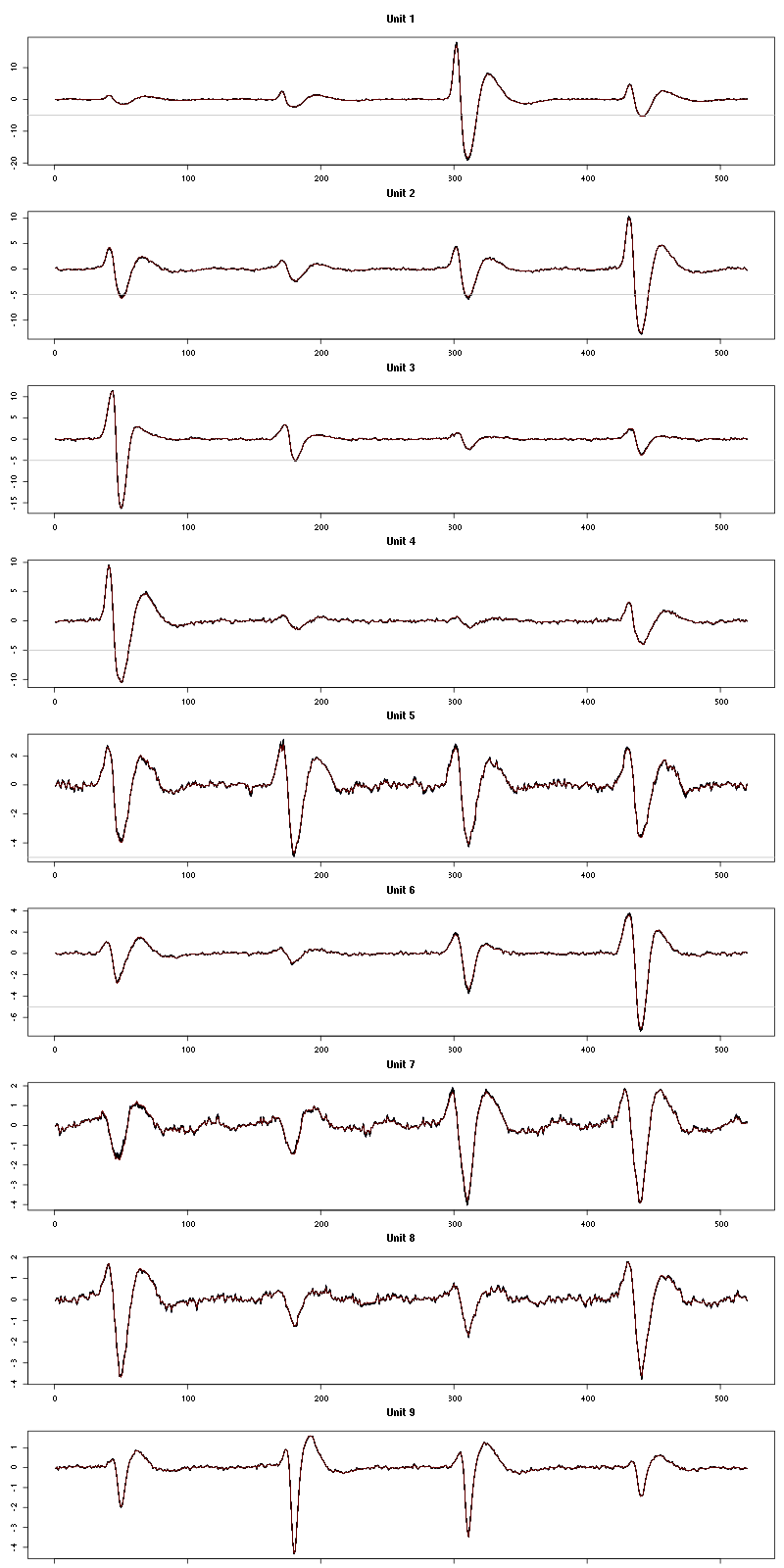
Figure 12: Evolution of the templates of each unit during the 50 trials with "pure" Cis_3_Hexen_1_ol for tetrode D.

The observed counting processes, inter spike intervals densities and raster plots are:

cp_isi_raster(a_Cis_3_Hexen_1_ol_0_f_tetD)

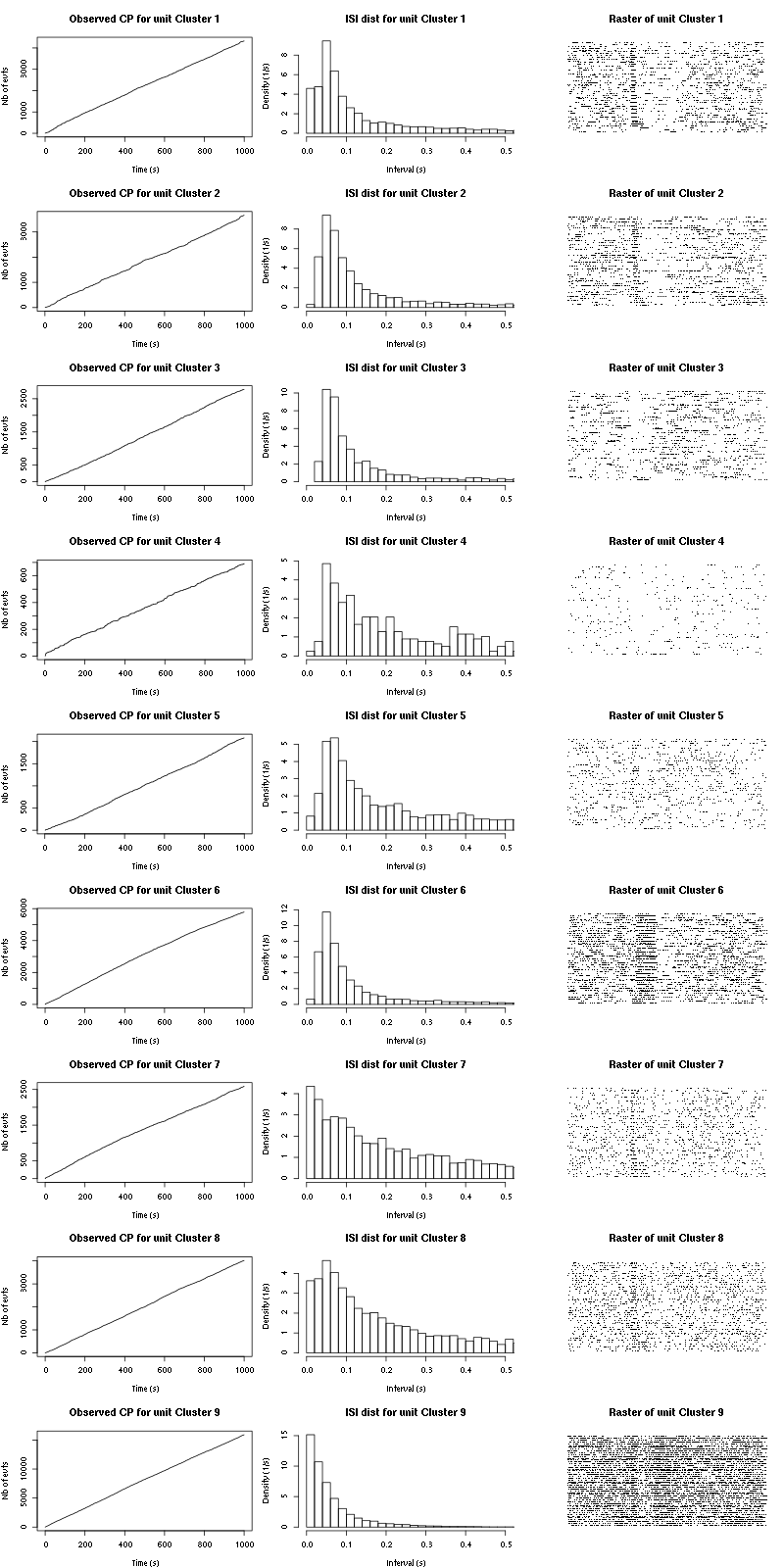
Figure 13: Observed counting processes, empirical inter spike interval distributions and raster plots for "pure" Cis_3_Hexen_1_ol.

4.3 Save results

Before analyzing the next set of trials we save the output of sort_many_trials to disk with:

save(a_Cis_3_Hexen_1_ol_0_f_tetD,
     file=paste0("tetD_analysis/tetD_","Cis_3_Hexen_1_ol_0_f","_summary_obj.rda"))

We write to disk the spike trains in text mode:

for (c_idx in 1:length(a_Cis_3_Hexen_1_ol_0_f_tetD$spike_trains))
    cat(a_Cis_3_Hexen_1_ol_0_f_tetD$spike_trains[[c_idx]],
        file=paste0("locust20000613_spike_trains/locust20000613_Cis_3_Hexen_1_ol_0_f_tetD_u",c_idx,".txt"),sep="\n")

5 10 remaining trials with `Cis-3-Hexen-1-ol` diluted 100 times

As mentioned in the LabBook, there are only 10 remaining trials among 50.

5.1 Do the job

We only write the command in the html file, not its output, the diagnostic plots in the next subsection should be enough to judge if everything went fine or not.

a_Cis_3_Hexen_1_ol_2_tetD=smt(stim_name="Cis-3-Hexen-1-ol (10^-2)",
                              trial_nbs=1:10,
                              centers=a_Cis_3_Hexen_1_ol_0_f_tetD$centers,
                              counts=a_Cis_3_Hexen_1_ol_0_f_tetD$counts)

5.2 Diagnostic plots

The counts evolution is:

counts_evolution(a_Cis_3_Hexen_1_ol_2_tetD)

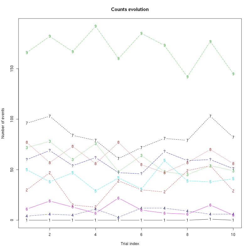
Figure 14: Evolution of the number of events attributed to each unit (1 to 10) or unclassified ("?") during the 10 remaining trials Cis_3_Hexen_1_ol diluted 100 times for tetrode D.

We see that the number of unclassified events increased a lot while the number of events attributed to unit 1 fell to zero. This suggests that we should re-estimate our model.

5.3 Model adjustment

We load data from the first trial:

lD = get_data(1,"Cis-3-Hexen-1-ol (10^-2)",
              channels = c("ch10","ch12","ch14","ch15"),
              file="locust20000613.hdf5")

We call all_at_once on these data as our function smt did:

at1d100=all_at_once(data=lD, a_Cis_3_Hexen_1_ol_0_f_tetD$centers,
                    thres=threshold_factor*c(1,1,1,1), 
                    filter_length_1=filter_length, filter_length=filter_length, 
                    minimalDist_1=15, minimalDist=15, 
                    before=c_before, after=c_after, 
                    detection_cycle=c(0,0), verbose=2)

The five number summary is:
      ch10           ch12           ch14           ch15     
 Min.   : 977   Min.   : 852   Min.   :1306   Min.   : 876  
 1st Qu.:2008   1st Qu.:1964   1st Qu.:2006   1st Qu.:1988  
 Median :2051   Median :2052   Median :2050   Median :2053  
 Mean   :2048   Mean   :2047   Mean   :2047   Mean   :2050  
 3rd Qu.:2091   3rd Qu.:2136   3rd Qu.:2092   3rd Qu.:2116  
 Max.   :2689   Max.   :2764   Max.   :2612   Max.   :3085  

Doing now round 0 detecting on all sites
    Total Cluster 1 Cluster 2 Cluster 3 Cluster 4 Cluster 5 Cluster 6 Cluster 7 
      454         0        30        72         4        50        11        92 
Cluster 8 Cluster 9         ? 
       64       130         1 

Doing now round 1 detecting on all sites
    Total Cluster 1 Cluster 2 Cluster 3 Cluster 4 Cluster 5 Cluster 6 Cluster 7 
      102         0         0         0         0         0         0         4 
Cluster 8 Cluster 9         ? 
       13        36        49 

Global counts at classification's end:
    Total Cluster 1 Cluster 2 Cluster 3 Cluster 4 Cluster 5 Cluster 6 Cluster 7 
      566         0        30        72         4        50        11        96 
Cluster 8 Cluster 9         ? 
       77       166        60

We can see all the detected but not classified events with:

at1d100$unknown

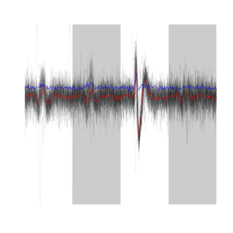
Figure 15: The 60 unclassified event from the first trial with Cis-3-Hexen-1-ol diluted 100 times

It is somehow a candidate for the former unit 1 since it generates large events only on the third site. So let us make long cuts from it.

new1pos = numeric(sum(sapply(at1d100$classification, function(c) c[[1]] == "?")))
nidx = 1
for (c in at1d100$classification)
    if (c[[1]] == "?") {
        new1pos[nidx] = c[[2]]
        nidx = nidx+1}
c1 = mk_center_list(new1pos,at1d100$residual+at1d100$prediction,before=c_before,after=c_after)
new_centers = a_Cis_3_Hexen_1_ol_0_f_tetD$centers
new_centers[[1]] = c1

Let's run all_at_once with new_centers:

at1d100=all_at_once(data=lD, new_centers,
                    thres=threshold_factor*c(1,1,1,1), 
                    filter_length_1=filter_length, filter_length=filter_length, 
                    minimalDist_1=15, minimalDist=15, 
                    before=c_before, after=c_after, 
                    detection_cycle=c(0,0), verbose=2)

The five number summary is:
      ch10           ch12           ch14           ch15     
 Min.   : 977   Min.   : 852   Min.   :1306   Min.   : 876  
 1st Qu.:2008   1st Qu.:1964   1st Qu.:2006   1st Qu.:1988  
 Median :2051   Median :2052   Median :2050   Median :2053  
 Mean   :2048   Mean   :2047   Mean   :2047   Mean   :2050  
 3rd Qu.:2091   3rd Qu.:2136   3rd Qu.:2092   3rd Qu.:2116  
 Max.   :2689   Max.   :2764   Max.   :2612   Max.   :3085  

Doing now round 0 detecting on all sites
    Total Cluster 1 Cluster 2 Cluster 3 Cluster 4 Cluster 5 Cluster 6 Cluster 7 
      454        87        30        72         4        13        11        42 
Cluster 8 Cluster 9         ? 
       64       130         1 

Doing now round 1 detecting on all sites
    Total Cluster 1 Cluster 2 Cluster 3 Cluster 4 Cluster 5 Cluster 6 Cluster 7 
       46         4         0         0         0         0         0         1 
Cluster 8 Cluster 9         ? 
       12        23         6 

Global counts at classification's end:
    Total Cluster 1 Cluster 2 Cluster 3 Cluster 4 Cluster 5 Cluster 6 Cluster 7 
      507        91        30        72         4        13        11        43 
Cluster 8 Cluster 9         ? 
       76       153        14

That looks much better! So we redo the analysis of the 10 trials with this new model.

5.4 Do the job with new model

a_Cis_3_Hexen_1_ol_2_tetD=smt(stim_name="Cis-3-Hexen-1-ol (10^-2)",
                              trial_nbs=1:10,
                              centers=new_centers,
                              counts=a_Cis_3_Hexen_1_ol_0_f_tetD$counts)

5.5 Diagnostic plots

The counts evolution is:

counts_evolution(a_Cis_3_Hexen_1_ol_2_tetD)

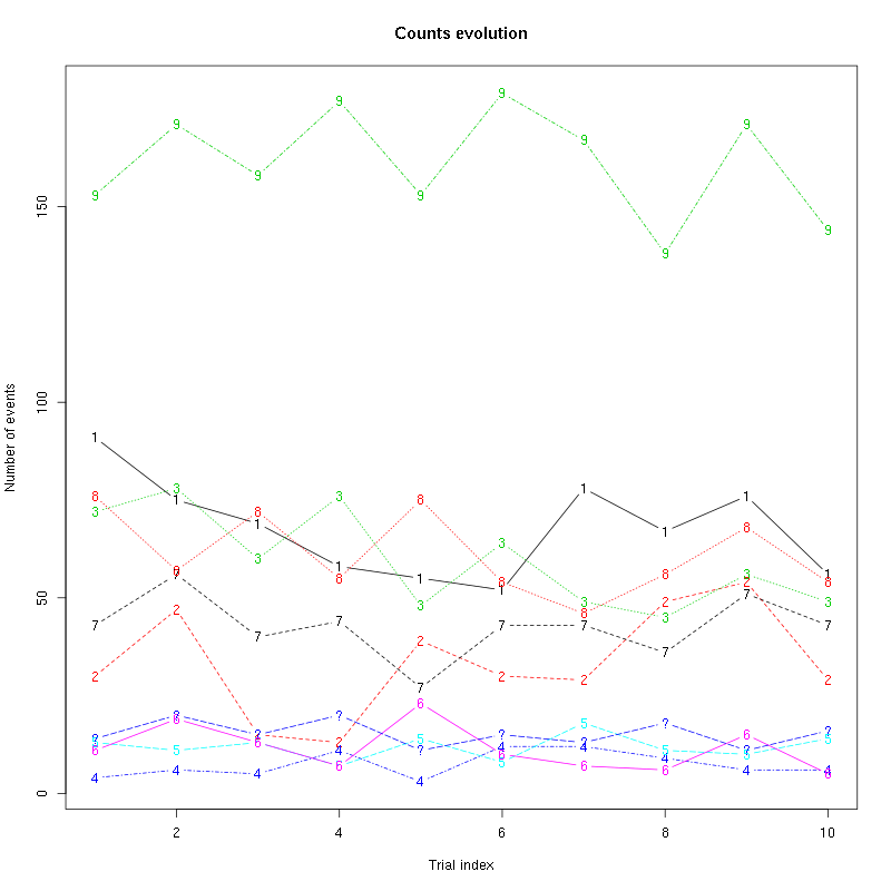
Figure 16: Evolution of the number of events attributed to each unit (1 to 10) or unclassified ("?") during the 10 remaining trials Cis_3_Hexen_1_ol diluted 100 times for tetrode D.

The waveform evolution is:

waveform_evolution(a_Cis_3_Hexen_1_ol_2_tetD,threshold_factor)

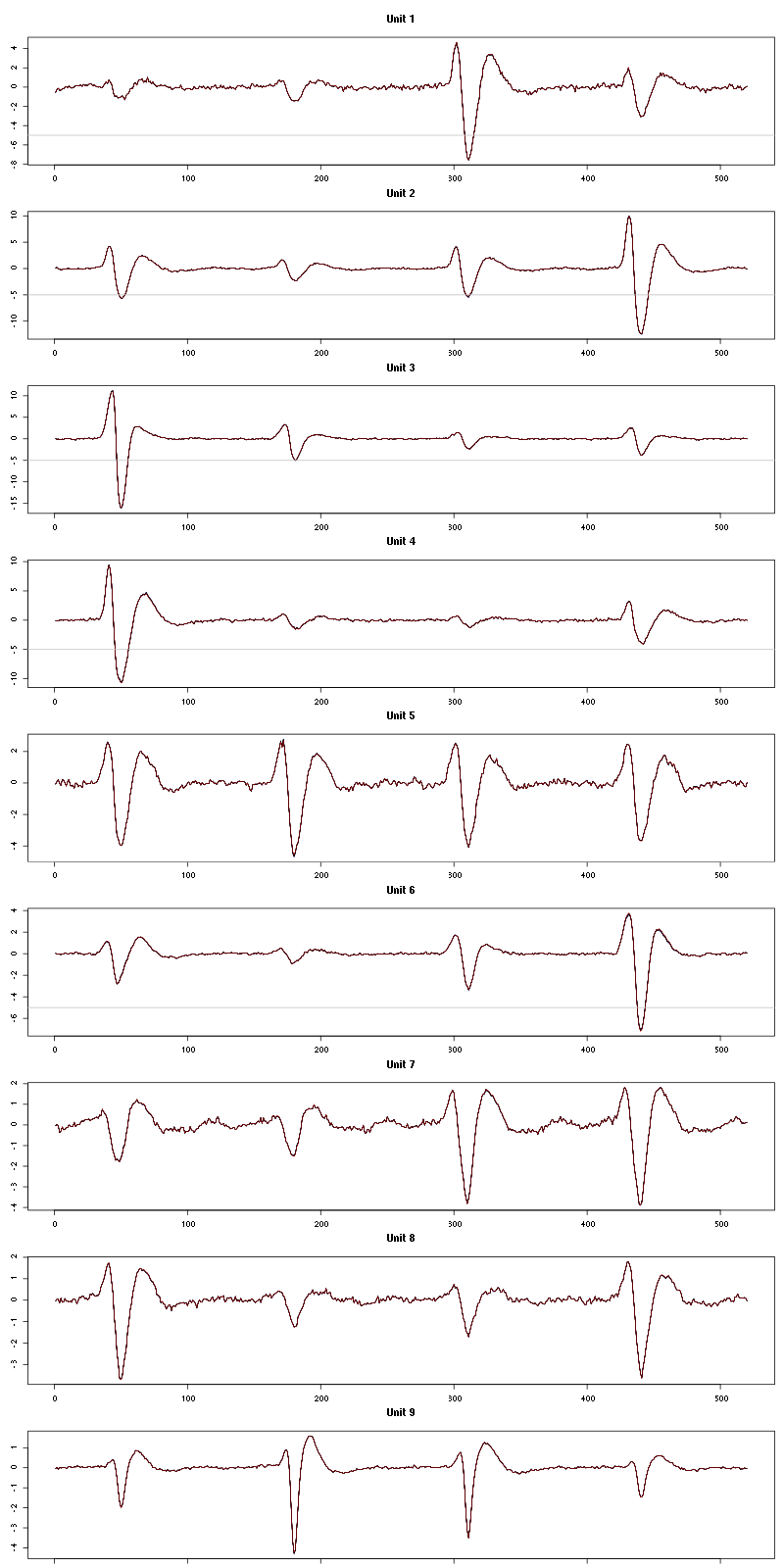
Figure 17: Evolution of the templates of each unit during the 10 remaining trials Cis_3_Hexen_1_ol diluted 100 times for tetrode D.

The observed counting processes, inter spike intervals densities and raster plots are:

cp_isi_raster(a_Cis_3_Hexen_1_ol_2_tetD)

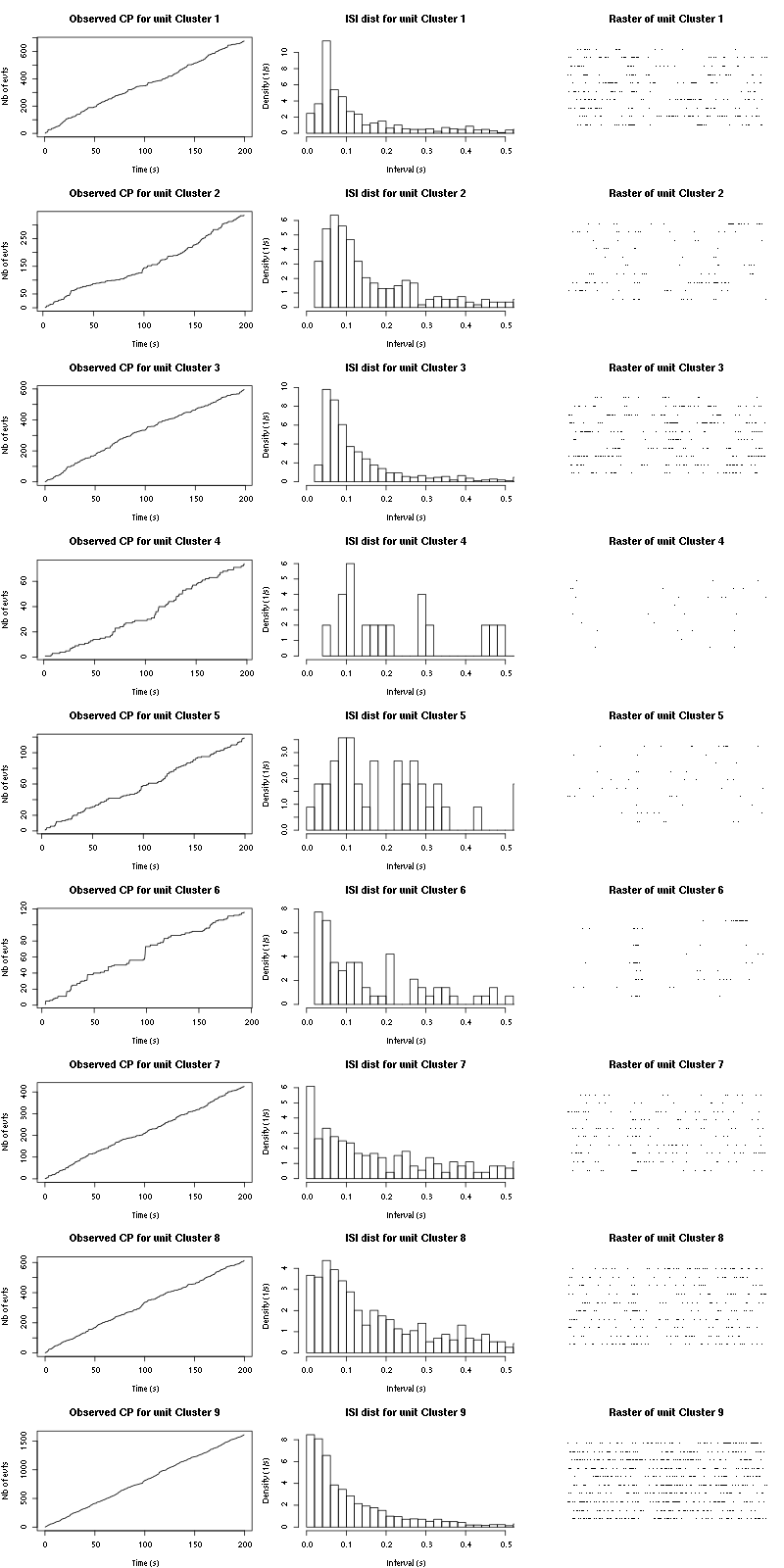
Figure 18: Observed counting processes, empirical inter spike interval distributions and raster plots for the 10 remaining trials Cis_3_Hexen_1_ol diluted 100 times for tetrode D.

5.6 Save results

Before analyzing the next set of trials we save the output of sort_many_trials to disk with:

save(a_Cis_3_Hexen_1_ol_2_tetD,
     file=paste0("tetD_analysis/tetD_","Cis_3_Hexen_1_ol_2","_summary_obj.rda"))

We write to disk the spike trains in text mode:

for (c_idx in 1:length(a_Cis_3_Hexen_1_ol_2_tetD$spike_trains))
    cat(a_Cis_3_Hexen_1_ol_2_tetD$spike_trains[[c_idx]],
        file=paste0("locust20000613_spike_trains/locust20000613_Cis_3_Hexen_1_ol_2_tetD_u",c_idx,".txt"),sep="\n")

6 50 trials with `Cis-3-hexen-1-ol` diluted 10 times

6.1 Do the job

stim_name = "Cis-3-Hexen-1-ol (10^-1)"
a_Cis_3_Hexen_1_ol_1_tetD=smt(stim_name=stim_name,
                              trial_nbs=1:50,
                              centers=a_Cis_3_Hexen_1_ol_2_tetD$centers,
                              counts=a_Cis_3_Hexen_1_ol_2_tetD$counts)

6.2 Diagnostic plots

The counts evolution is:

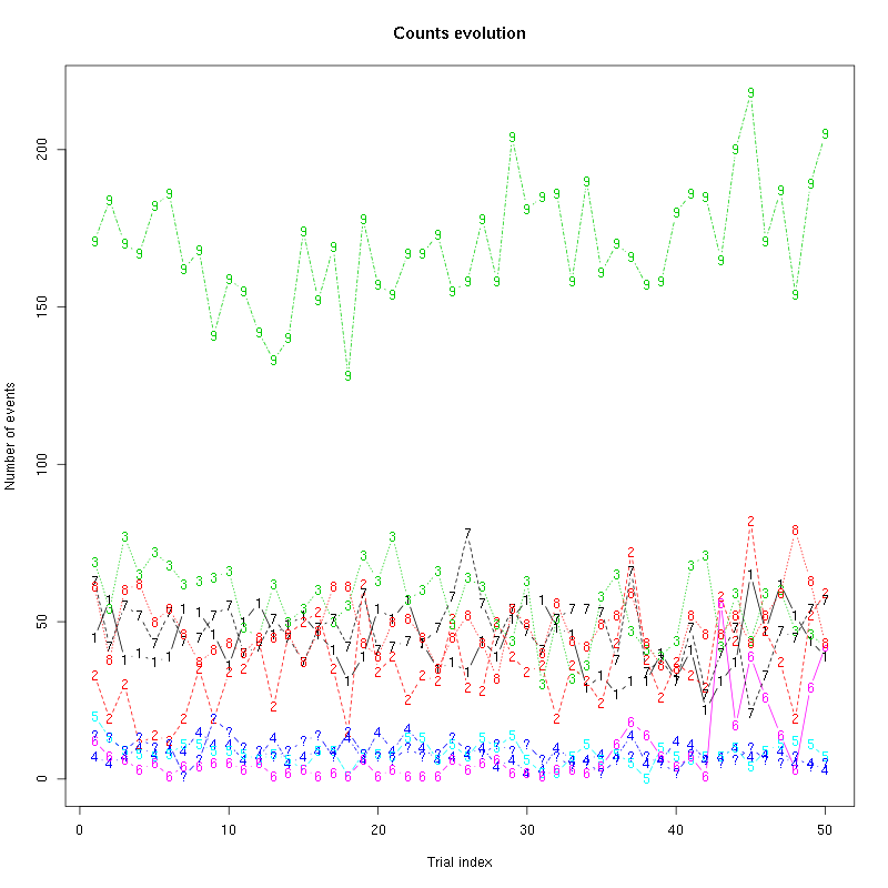
Figure 19: Evolution of the number of events attributed to each unit (1 to 9) or unclassified ("?") during the 50 trials of Cis-3-Hexen-1-ol diluted 10 times for tetrodeD.

The waveform evolution is:

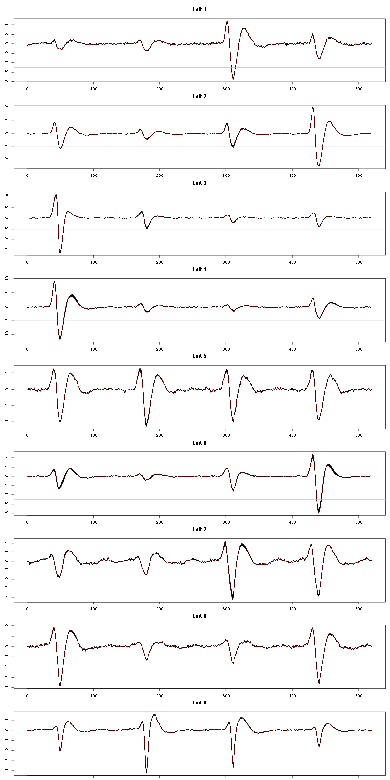
Figure 20: Evolution of the templates of each unit during the 50 trials of Cis-3-Hexen-1-ol diluted 10 times for tetrodeD.

The observed counting processes, inter spike intervals densities and raster plots are:

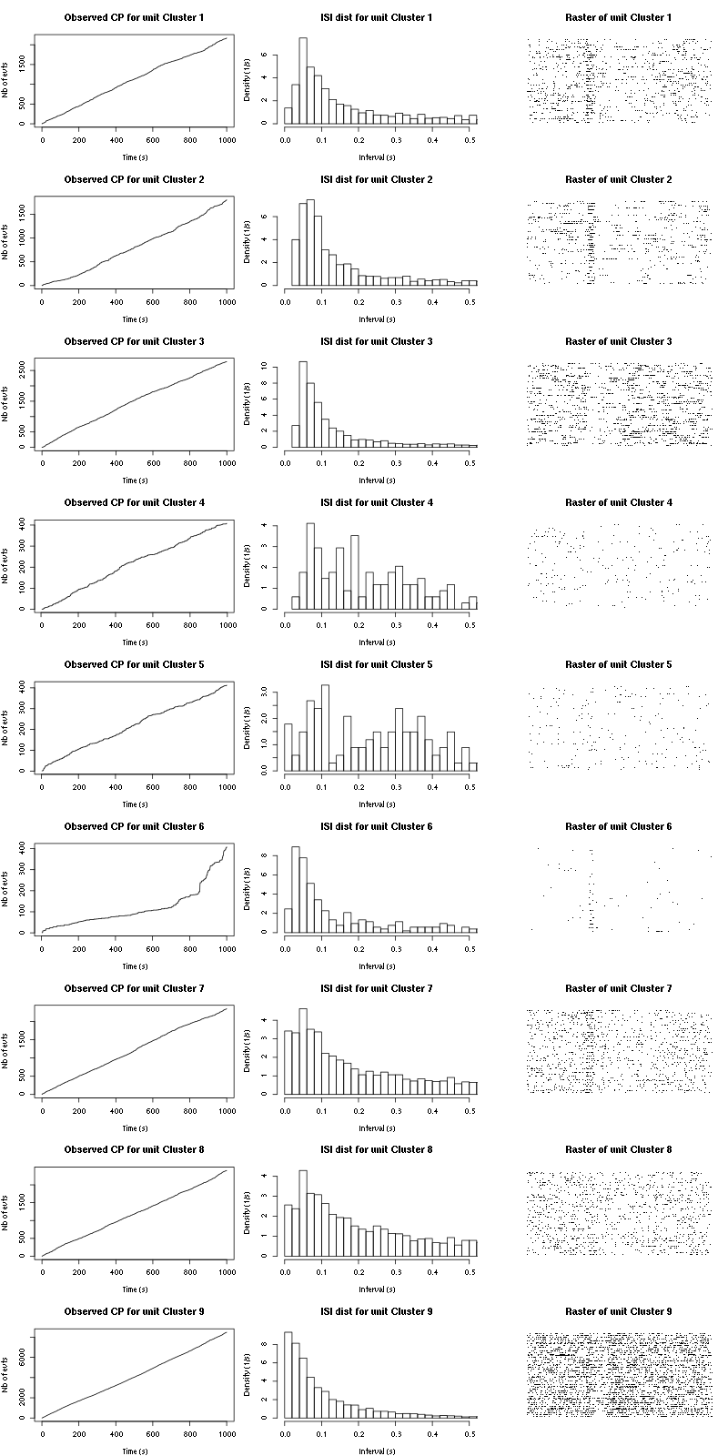
Figure 21: Observed counting processes, empirical inter spike interval distributions and raster plots during the 60 trials of Cis_3_Hexen_1_ol_1 for tetrodeD.

6.3 Save results

Before analyzing the next set of trials we save the output of sort_many_trials to disk with:

save(a_Cis_3_Hexen_1_ol_1_tetD,
     file=paste0("tetD_analysis/tetD_",stim_name,"_summary_obj.rda"))

We write to disk the spike trains in text mode:

for (c_idx in 1:length(a_Cis_3_Hexen_1_ol_1_tetD$spike_trains))
    if (!is.null(a_Cis_3_Hexen_1_ol_1_tetD$spike_trains[[c_idx]]))
        cat(a_Cis_3_Hexen_1_ol_1_tetD$spike_trains[[c_idx]],file=paste0("locust20000613_spike_trains/locust20000613_Cis_3_Hexen_1_ol_1_tetD_u",c_idx,".txt"),sep="\n")

7 Systematic analysis of the second set of 50 trials with "pure" `Cis-3-Hexen-1-ol`

7.1 Doing the job

a_Cis_3_Hexen_1_ol_0_s_tetD=smt(stim_name="Cis-3-Hexen-1-ol (10^-0) second",
                                trial_nbs=1:50,
                                centers=a_Cis_3_Hexen_1_ol_1_tetD$centers,
                                counts=a_Cis_3_Hexen_1_ol_1_tetD$counts)

7.2 Diagnostic plots

The counts evolution is:

counts_evolution(a_Cis_3_Hexen_1_ol_0_s_tetD)

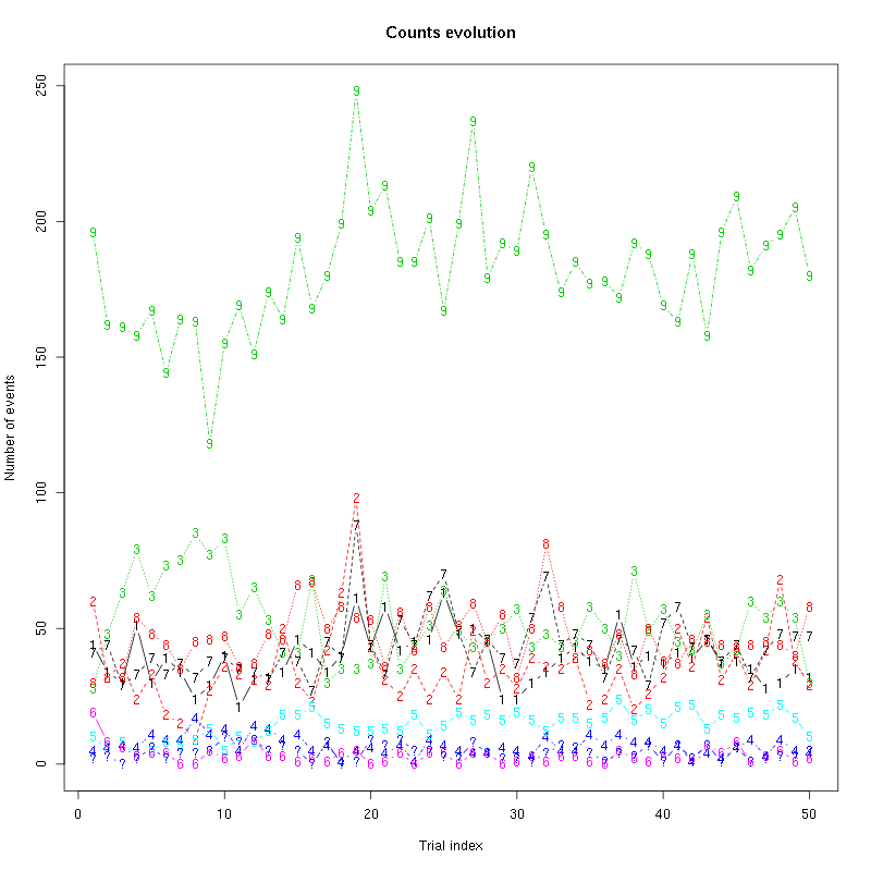
Figure 22: Evolution of the number of events attributed to each unit (1 to 9) or unclassified ("?") during the second group of 50 trials with "pure" Cis_3_Hexen_1_ol for tetrode D.

The waveform evolution is:

waveform_evolution(a_Cis_3_Hexen_1_ol_0_s_tetD,threshold_factor)

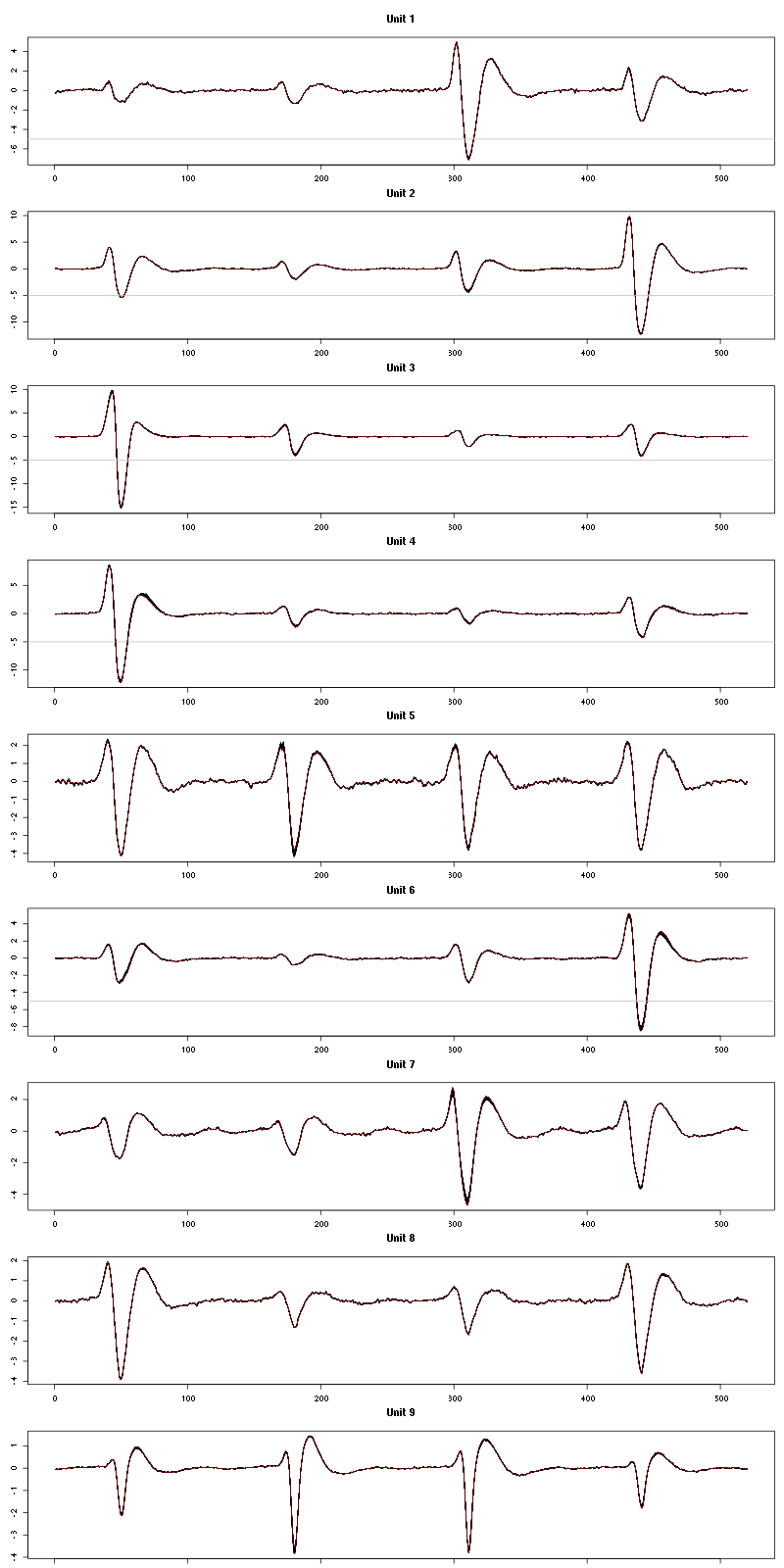
Figure 23: Evolution of the templates of each unit during the second group of 50 trials with "pure" Cis_3_Hexen_1_ol for tetrode D.

The observed counting processes, inter spike intervals densities and raster plots are:

cp_isi_raster(a_Cis_3_Hexen_1_ol_0_s_tetD)

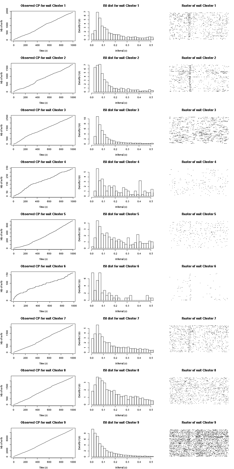
Figure 24: Observed counting processes, empirical inter spike interval distributions and raster plots during the second group of 50 trials with "pure" Cis_3_Hexen_1_ol.

7.3 Save results

Before analyzing the next set of trials we save the output of sort_many_trials to disk with:

save(a_Cis_3_Hexen_1_ol_0_s_tetD,
     file=paste0("tetD_analysis/tetD_","Cis_3_Hexen_1_ol_0_s","_summary_obj.rda"))

We write to disk the spike trains in text mode:

for (c_idx in 1:length(a_Cis_3_Hexen_1_ol_0_s_tetD$spike_trains))
    cat(a_Cis_3_Hexen_1_ol_0_s_tetD$spike_trains[[c_idx]],
        file=paste0("locust20000613_spike_trains/locust20000613_Cis_3_Hexen_1_ol_0_s_tetD_u",c_idx,".txt"),sep="\n")

8 Systematic analysis of the second set of 20 trials with `Cherry`

8.1 Doing the job

a_Cherry_tetD=smt(stim_name="Cherry",
                  trial_nbs=1:20,
                  centers=a_Cis_3_Hexen_1_ol_0_s_tetD$centers,
                  counts=a_Cis_3_Hexen_1_ol_0_s_tetD$counts)

8.2 Diagnostic plots

The counts evolution is:

counts_evolution(a_Cherry_tetD)

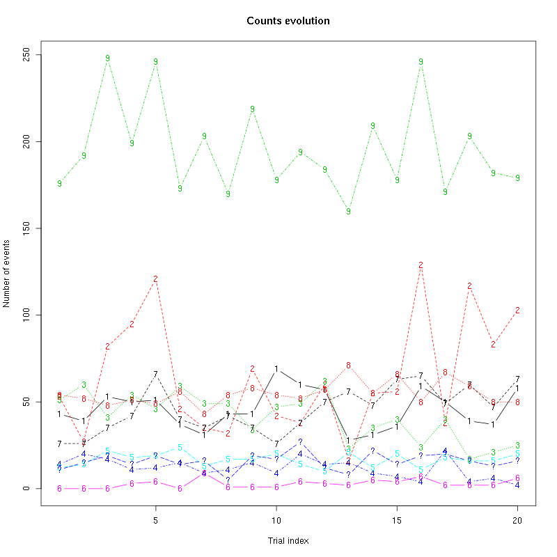
Figure 25: Evolution of the number of events attributed to each unit (1 to 9) or unclassified ("?") during the 20 trials with Cherry for tetrode D.

The waveform evolution is:

waveform_evolution(a_Cherry_tetD,threshold_factor)

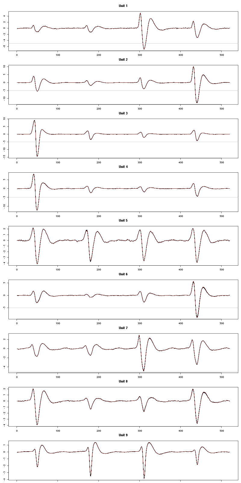
Figure 26: Evolution of the templates of each unit during the 20 trials with Cherry for tetrode D.

The observed counting processes, inter spike intervals densities and raster plots are:

cp_isi_raster(a_Cherry_tetD)

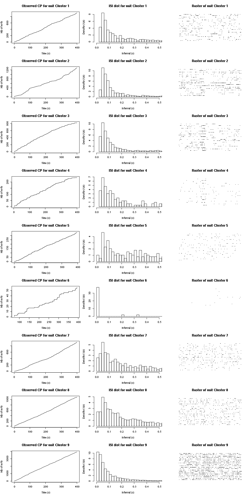
Figure 27: Observed counting processes, empirical inter spike interval distributions and raster plots during the 20 trials with Cherry.

8.3 Save results

Before analyzing the next set of trials we save the output of sort_many_trials to disk with:

save(a_Cherry_tetD,
     file=paste0("tetD_analysis/tetD_","Cherry","_summary_obj.rda"))

We write to disk the spike trains in text mode:

for (c_idx in 1:length(a_Cherry_tetD$spike_trains))
    cat(a_Cherry_tetD$spike_trains[[c_idx]],
        file=paste0("locust20000613_spike_trains/locust20000613_Cherry_tetD_u",c_idx,".txt"),sep="\n")

Sorting data set 20000613 tetrode D (channels 10, 12, 14, 15)

Table of Contents

1 Introduction

1.1 Getting the data

1.2 Getting the code

2 Tetrode D (channels 10, 12, 14, 15) analysis

2.1 Loading the data

2.2 Five number summary

2.3 Plot the data

2.4 Data normalization

2.5 Spike detection

2.6 Cuts

2.7 Events

2.8 Removing obvious superposition

2.9 Dimension reduction

2.10 Exporting for GGobi

2.11 kmeans clustering with 9

2.12 Long cuts creation

2.13 Peeling

2.13.1 Round 0

2.13.2 Round 1

2.13.3 Round 2

2.14 Getting the spike trains

2.15 Getting the inter spike intervals and the forward and backward recurrence times

2.15.1 ISI distributions

2.15.2 Forward and Backward Recurrence Times

2.16 Testing all_at_once

3 Analyzing a sequence of trials

3.1 Create directories were results get saved

3.2 Define a "taylored" version of sort_many_trials

4 Systematic analysis of the 50 trials with "pure" Cis-3-Hexen-1-ol

4.1 Doing the job

4.2 Diagnostic plots

4.3 Save results

5 10 remaining trials with Cis-3-Hexen-1-ol diluted 100 times

5.1 Do the job

5.2 Diagnostic plots

5.3 Model adjustment

5.4 Do the job with new model

5.5 Diagnostic plots

5.6 Save results

6 50 trials with Cis-3-hexen-1-ol diluted 10 times

6.1 Do the job

6.2 Diagnostic plots

6.3 Save results

7 Systematic analysis of the second set of 50 trials with "pure" Cis-3-Hexen-1-ol

7.1 Doing the job

7.2 Diagnostic plots

7.3 Save results

8 Systematic analysis of the second set of 20 trials with Cherry

8.1 Doing the job

8.2 Diagnostic plots

8.3 Save results

2.10 Exporting for `GGobi`

2.16 Testing `all_at_once`

3.2 Define a "taylored" version of `sort_many_trials`

4 Systematic analysis of the 50 trials with "pure" `Cis-3-Hexen-1-ol`

5 10 remaining trials with `Cis-3-Hexen-1-ol` diluted 100 times

6 50 trials with `Cis-3-hexen-1-ol` diluted 10 times

7 Systematic analysis of the second set of 50 trials with "pure" `Cis-3-Hexen-1-ol`

8 Systematic analysis of the second set of 20 trials with `Cherry`