Sorting data set 20010214 tetrode B (channels 2, 3, 5, 7)

1. Introduction
- 1.1. Getting the data
- 1.2. Getting the code
2. Tetrode B (channels 2, 3, 5, 7) analysis
3. Analyzing a sequence of trials
4. Systematic analysis of the 30 trials from Spontaneous_2 backwards
5. 30 trials of Spontaenous_1 backwards
6. 25 trials with Cis-3-Hexen-1-ol (C3H_1)
7. 25 trials with Citral
8. 25 trials with Vanilla
9. 25 trials with Octanol
10. 25 trials with Mint
11. 25 trials with C3H_2
12. 30 trials of Spontaneous_3
13. 30 trials of Spontaneous_4
14. 30 trials of C3H_3
15. 10 trials of C3H_4
16. 30 trials of C3H_5
17. 30 trials of C3H_6

1 Introduction

This is the description of how to do the (spike) sorting of tetrode B (channels 2, 3, 5, 7) from data set locust20010214.

1.1 Getting the data

The data are in file locust20010214.hdf5 located on zenodo and can be downloaded interactivelly with a web browser or by typing at the command line:

wget https://zenodo.org/record/21589/files/locust20010214_part1.hdf5
wget https://zenodo.org/record/21589/files/locust20010214_part2.hdf5

In the sequel I will assume that R has been started in the directory where the data were downloaded (in other words, the working direcory should be the one containing the data.

The data are in HDF5 format and the easiest way to get them into R is to install the rhdf5 package from Bioconductor. Once the installation is done, the library is loaded into R with:

library(rhdf5)

We can then get a (long and detailed) listing of our data file content with (result not shown):

h5ls("locust20010214_part1.hdf5")

We can get the content of LabBook metadata from the shell with:

h5dump -a "LabBook" locust20010214_part1.hdf5

1.2 Getting the code

The code can be sourced as follows:

source("https://raw.githubusercontent.com/christophe-pouzat/zenodo-locust-datasets-analysis/master/R_Sorting_Code/sorting_with_r.R")

A description of the functions contained in this file can be found at the following address: http://xtof.perso.math.cnrs.fr/locust.html.

2 Tetrode B (channels 2, 3, 5, 7) analysis

We now want to get our "model", that is a dictionnary of waveforms (one waveform per neuron and per recording site). To that end we are going to use the last 60 s of data contained in the Spontaneous_2 Group (in HDF5 jargon).

2.1 Loading the data

So we start by loading the data from channels 2, 3, 5, 7 into R:

lD = rbind(cbind(h5read("locust20010214_part1.hdf5", "/Spontaneous_2/trial_30/ch02"),
                 h5read("locust20010214_part1.hdf5", "/Spontaneous_2/trial_30/ch03"),
                 h5read("locust20010214_part1.hdf5", "/Spontaneous_2/trial_30/ch05"),
                 h5read("locust20010214_part1.hdf5", "/Spontaneous_2/trial_30/ch07")))
dim(lD)

431548

2.2 Five number summary

We get the Five number summary with:

summary(lD,digits=2)

Min. : 98	Min. : 610	Min. : 762	Min. : 475
1st Qu.:2011	1st Qu.:2015	1st Qu.:2017	1st Qu.:2014
Median :2058	Median :2057	Median :2057	Median :2059
Mean :2055	Mean :2055	Mean :2054	Mean :2056
3rd Qu.:2105	3rd Qu.:2099	3rd Qu.:2095	3rd Qu.:2102
Max. :3634	Max. :3076	Max. :2887	Max. :3143

It shows that the channels have very similar properties as far as the median and the inter-quartile range (IQR) are concerned. The minimum is much smaller on the first channel. This suggests that the largest spikes are going to be found here (remember that spikes are going mainly downwards).

2.3 Plot the data

We "convert" the data matrix lD into a time series object with:

lD = ts(lD,start=0,freq=15e3)

We can then plot the whole data with (not shown since it makes a very figure):

plot(lD)

2.4 Data normalization

As always we normalize such that the median absolute deviation (MAD) becomes 1:

lD.mad = apply(lD,2,mad)
lD = t((t(lD)-apply(lD,2,median))/lD.mad)
lD = ts(lD,start=0,freq=15e3)

Once this is done we explore interactively the data with:

explore(lD,col=c("black","grey70"))

Most spikes can be seen on the 4 recording sites, there are many different spike waveform and the signal to noise ratio is really good!

2.5 Spike detection

Since the spikes are mainly going downwards, we will detect valleys instead of peaks:

lDf = -lD
filter_length = 5
threshold_factor = 4
lDf = filter(lDf,rep(1,filter_length)/filter_length)
lDf[is.na(lDf)] = 0
lDf.mad = apply(lDf,2,mad)
lDf_mad_original = lDf.mad
lDf = t(t(lDf)/lDf_mad_original)
thrs = threshold_factor*c(1,1,1,1)
bellow.thrs = t(t(lDf) < thrs)
lDfr = lDf
lDfr[bellow.thrs] = 0
remove(lDf)
sp0 = peaks(apply(lDfr,1,sum),15)
remove(lDfr)
sp0

eventsPos object with indexes of 1950 events. 
  Mean inter event interval: 221.2 sampling points, corresponding SD: 204.2 sampling points 
  Smallest and largest inter event intervals: 16 and 2904 sampling points.

Every time a filter length / threshold combination is tried, the detection is checked interactively with:

explore(sp0,lD,col=c("black","grey50"))

2.6 Cuts

We proceed as usual to get the cut length right:

evts = mkEvents(sp0,lD,49,50)
evts.med = median(evts)
evts.mad = apply(evts,1,mad)
plot_range = range(c(evts.med,evts.mad))
plot(evts.med,type="n",ylab="Amplitude",
     ylim=plot_range)
abline(v=seq(0,400,10),col="grey")
abline(h=c(0,1),col="grey")
lines(evts.med,lwd=2)
lines(evts.mad,col=2,lwd=2)

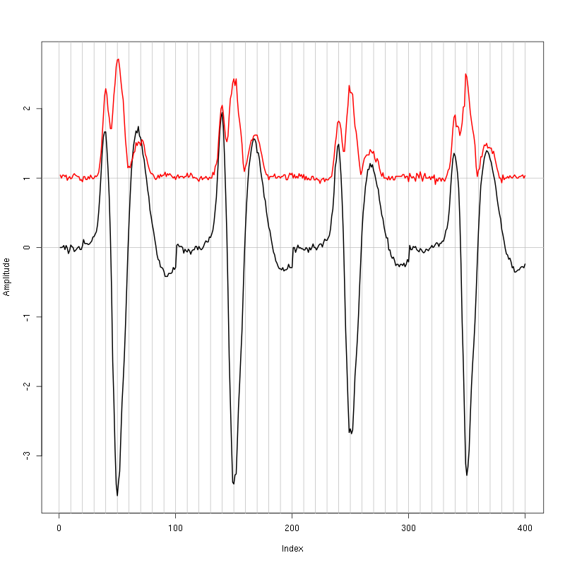
Figure 1: Setting the cut length for the data from tetrode B (channels 2, 3, 5, 7). We see that we need 20 points before the peak and 30 after.

We see that we need roughly 20 points before the peak and 30 after.

2.7 Events

We now cut our events:

evts = mkEvents(sp0,lD,19,30)
summary(evts)

events object deriving from data set: lD.
 Events defined as cuts of 50 sampling points on each of the 4 recording sites.
 The 'reference' time of each event is located at point 20 of the cut.
 There are 1950 events in the object.

We can as usual visualize the first 200 events with:

evts[,1:200]

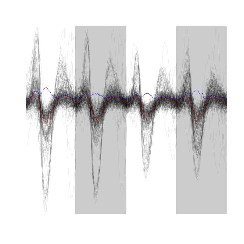
Figure 2: First 200 events for the data from tetrode B (channels 1, 3, 5, 7).

There are few superpositions so we try to remove the most obvious ones before doing the dimension reduction.

2.8 Removing obvious superposition

We define function goodEvtsFct with:

goodEvtsFct = function(samp,thr=3) {
    samp.med = apply(samp,1,median)
    samp.mad = apply(samp,1,mad)
    below = samp.med < 0
    samp.r = apply(samp,2,function(x) {x[below] = 0;x})
    apply(samp.r,2,function(x) all(abs(x-samp.med) < thr*samp.mad))
}

We apply it with a threshold of 8 times the MAD:

goodEvts = goodEvtsFct(evts,8)

2.9 Dimension reduction

We do a PCA on our good events set:

evts.pc = prcomp(t(evts[,goodEvts]))

We look at the projections on the first 4 principle components:

panel.dens = function(x,...) {
  usr = par("usr")
  on.exit(par(usr))
  par(usr = c(usr[1:2], 0, 1.5) )
  d = density(x, adjust=0.5)
  x = d$x
  y = d$y
  y = y/max(y)
  lines(x, y, col="grey50", ...)
}
pairs(evts.pc$x[,1:4],pch=".",gap=0,diag.panel=panel.dens)

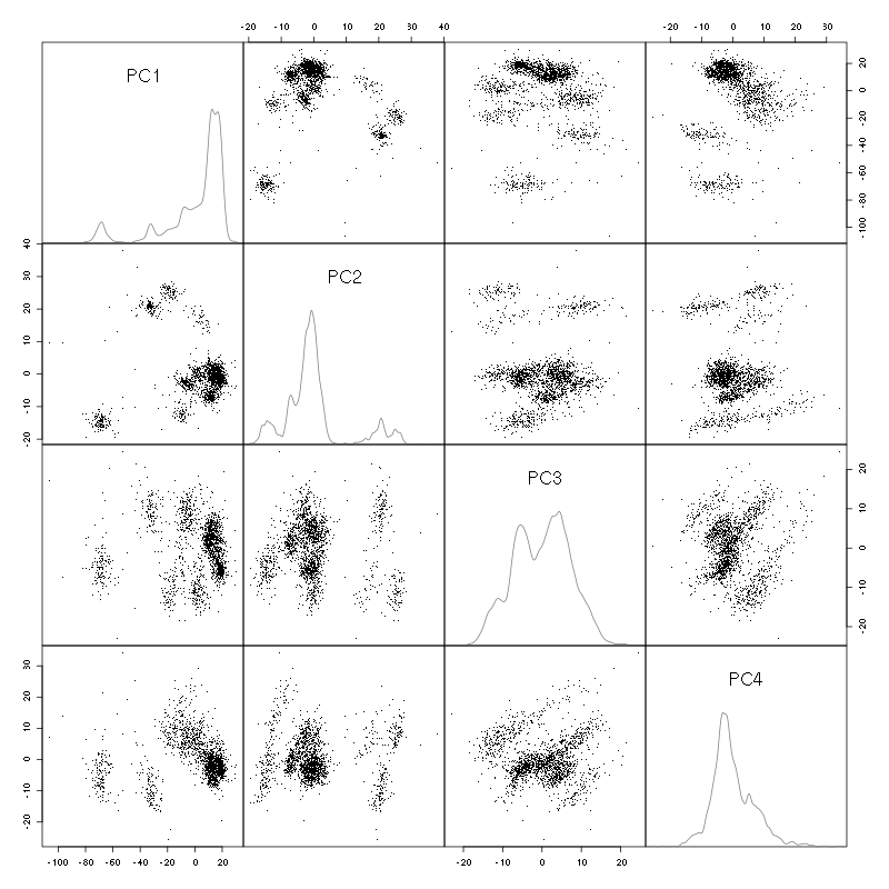
Figure 3: Events from tetrode B (channels 2, 3, 5, 7) projected onto the first 4 PCs.

I see at least 10 clusters. We can also look at the projections on the PC pairs defined by the next 4 PCs:

pairs(evts.pc$x[,5:8],pch=".",gap=0,diag.panel=panel.dens)

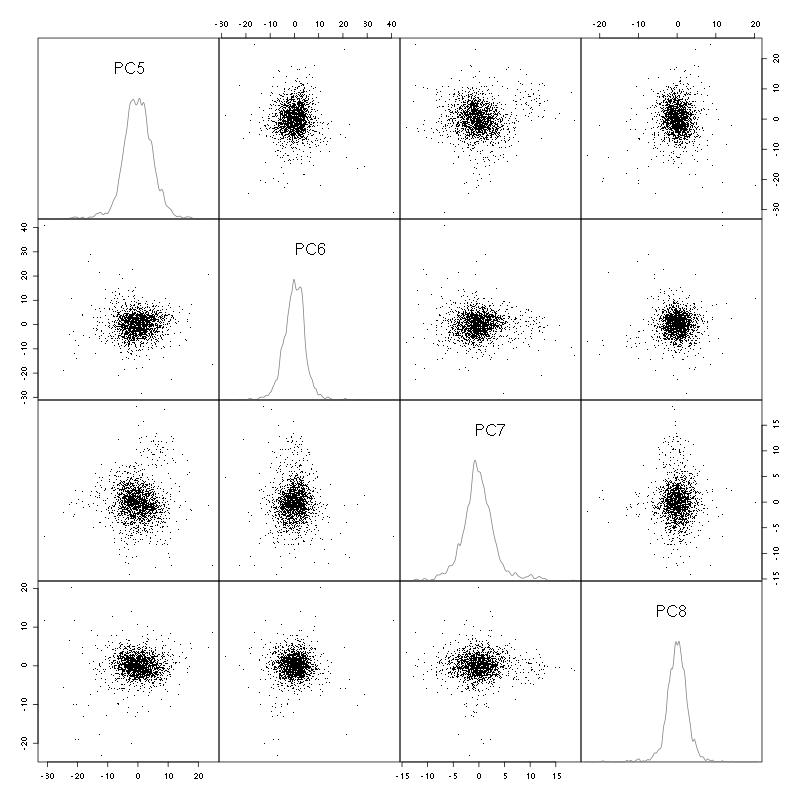
Figure 4: Events from tetrode B (channels 2, 3, 5, 7) projected onto PC 5 to 8.

There is not much structure left beyond the 4th PC.

2.10 Exporting for `GGobi`

We export the events projected onto the first 8 principle components in csv format:

write.csv(evts.pc$x[,1:8],file="tetB_evts.csv")

Using the rotation display of GGobi with the first 3 principle components and the 2D tour with the first 4 components I see at least 10. So we will start with a kmeans with 10 centers.

2.11 kmeans clustering with 10

nbc=10
set.seed(20110928,kind="Mersenne-Twister")
km = kmeans(evts.pc$x[,1:4],centers=nbc,iter.max=100,nstart=100)
label = km$cluster
cluster.med = sapply(1:nbc, function(cIdx) median(evts[,goodEvts][,label==cIdx]))
sizeC = sapply(1:nbc,function(cIdx) sum(abs(cluster.med[,cIdx])))
newOrder = sort.int(sizeC,decreasing=TRUE,index.return=TRUE)$ix
cluster.mad = sapply(1:nbc, function(cIdx) {ce = t(evts[,goodEvts]);ce = ce[label==cIdx,];apply(ce,2,mad)})
cluster.med = cluster.med[,newOrder]
cluster.mad = cluster.mad[,newOrder]
labelb = sapply(1:nbc, function(idx) (1:nbc)[newOrder==idx])[label]

We write a new csv file with the data and the labels:

write.csv(cbind(evts.pc$x[,1:4],labelb),file="tetB_sorted.csv")

It gives what was expected.

We get a plot showing the events attributed to each of the first 5 units with:

layout(matrix(1:5,nr=5))
par(mar=c(1,1,1,1))
for (i in (1:5)) plot(evts[,goodEvts][,labelb==i],y.bar=5)

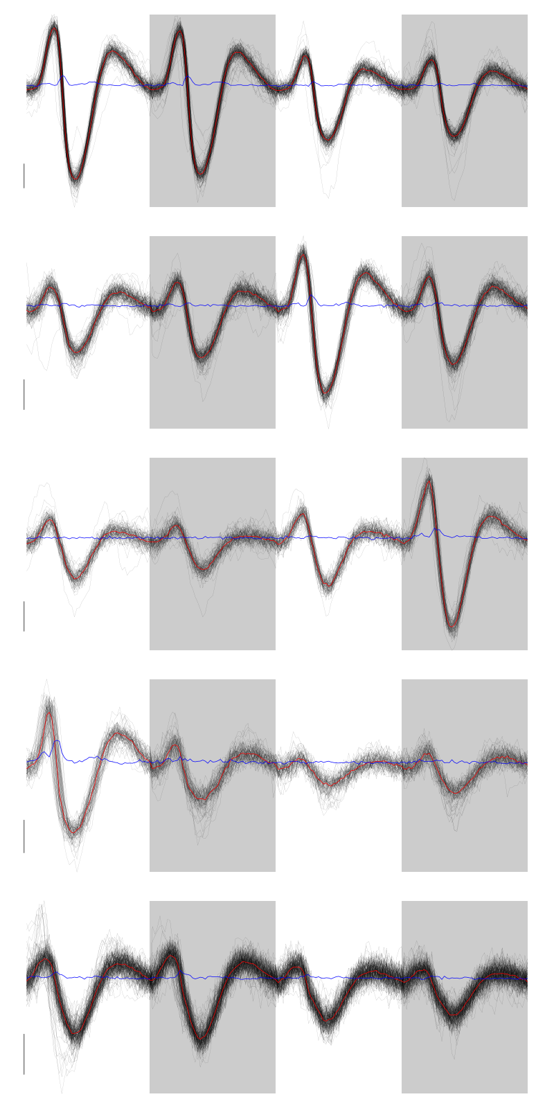
Figure 5: The events of the first five clusters of tetrode B

We get a plot showing the events attributed to each of the last 5 units with:

layout(matrix(1:5,nr=5))
par(mar=c(1,1,1,1))
for (i in (6:10)) plot(evts[,goodEvts][,labelb==i],y.bar=5)

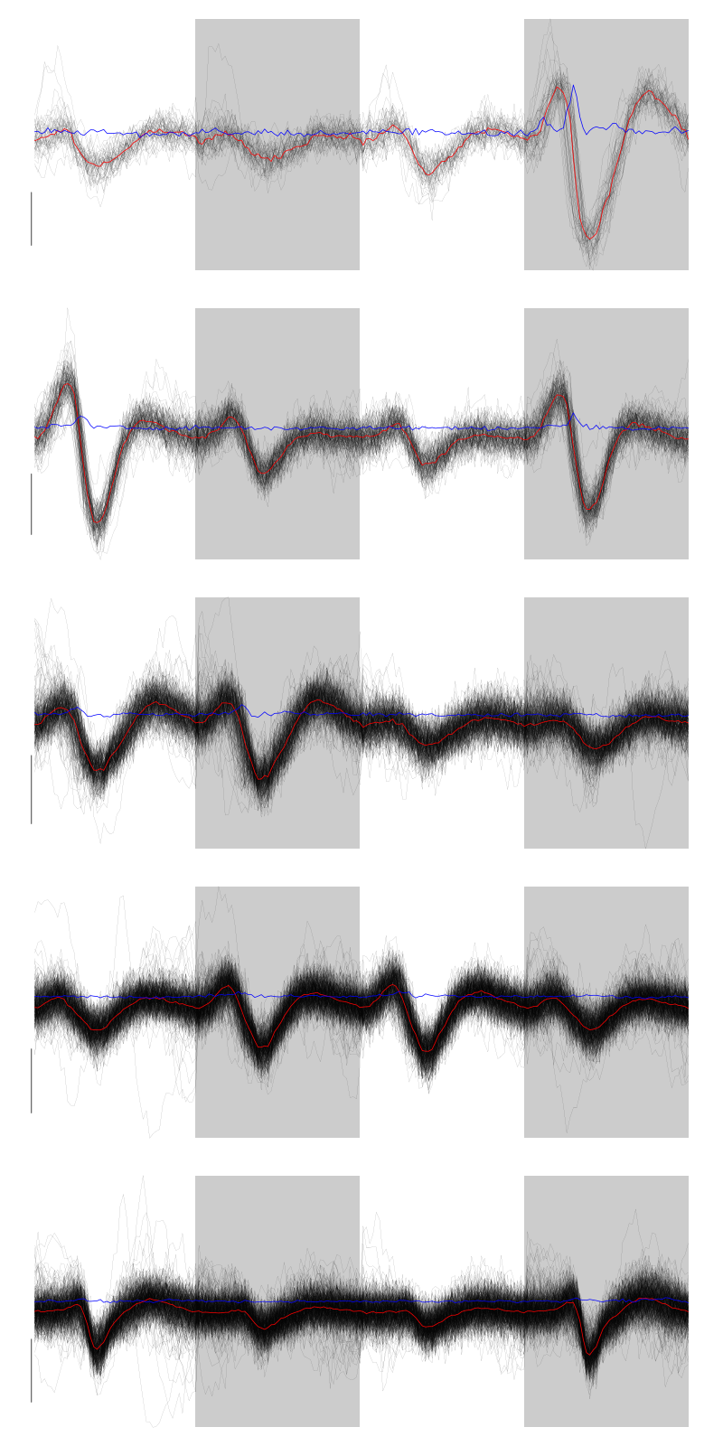
Figure 6: The events of the last five clusters of tetrode B

2.12 Long cuts creation

For the peeling process we need templates that start and end at 0 (we will otherwise generate artifacts when we subtract). We proceed "as usual" with (I tried first with the default value for parameters before and after but I reduced their values after looking at the centers, see the next figure):

c_before = 49
c_after = 80
centers = lapply(1:nbc, function(i)
    mk_center_list(sp0[goodEvts][labelb==i],lD,
                   before=c_before,after=c_after))
names(centers) = paste("Cluster",1:nbc)

We then make sure that our cuts are long enough by looking at them (the first 5):

layout(matrix(1:5,nr=5))
par(mar=c(1,4,1,1))
the_range=c(min(sapply(centers,function(l) min(l$center))),
            max(sapply(centers,function(l) max(l$center))))
for (i in 1:5) {
    template = centers[[i]]$center
    plot(template,lwd=2,col=2,
         ylim=the_range,type="l",ylab="")
    abline(h=0,col="grey50")
    abline(v=(1:2)*(c_before+c_after)+1,col="grey50")
    lines(filter(template,rep(1,filter_length)/filter_length),
          col=1,lty=3,lwd=2)
    abline(h=-threshold_factor,col="grey",lty=2,lwd=2)
    lines(centers[[i]]$centerD,lwd=2,col=4)
}

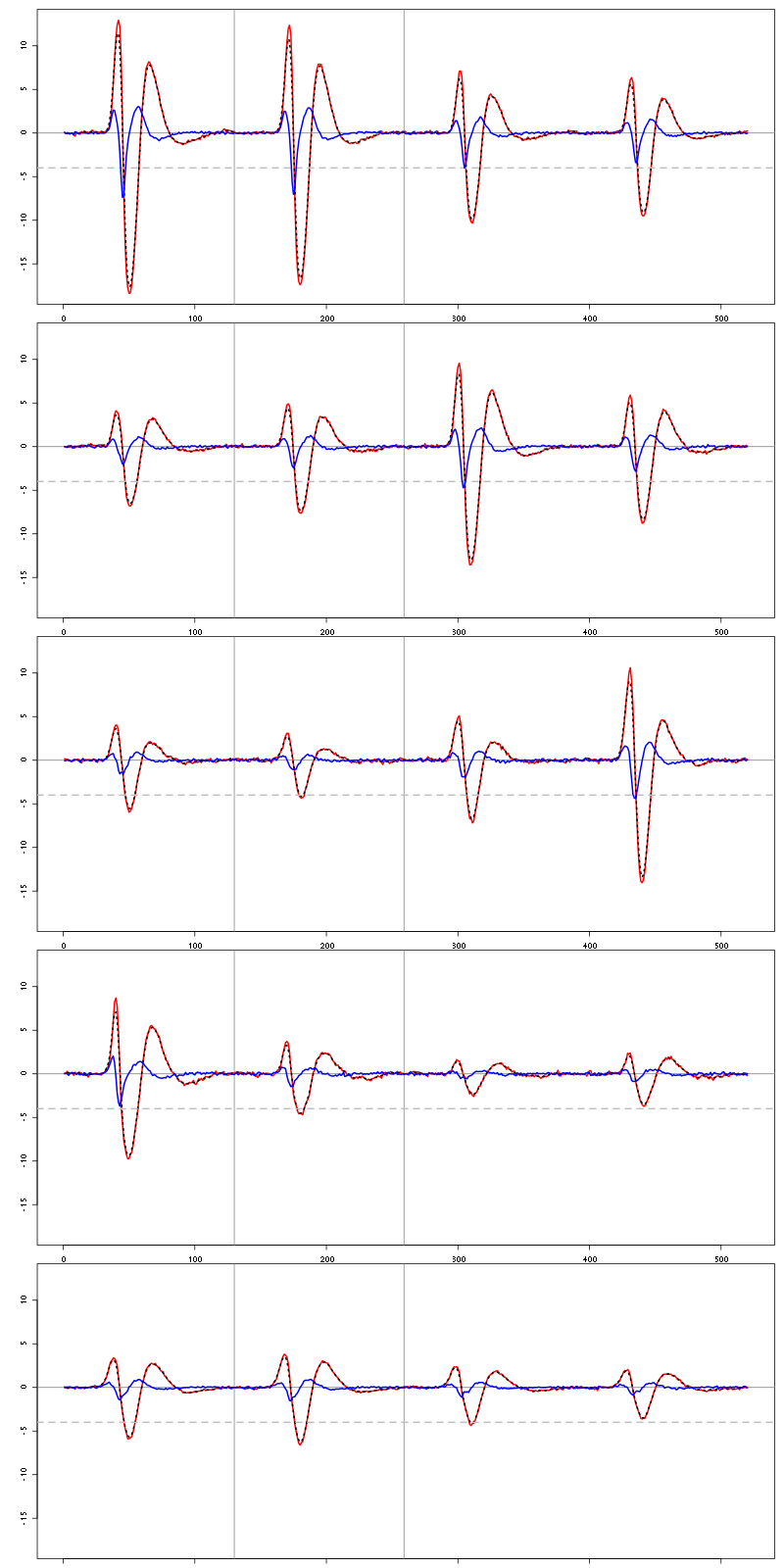
Figure 7: The first five templates (red) together with their first derivative (blue) all with the same scale. The dashed black curve show the templates filtered with the filter used during spike detection and the horizontal dashed grey line shows the detection threshold.

The last five:

layout(matrix(1:5,nr=5))
par(mar=c(1,4,1,1))
the_range=c(min(sapply(centers,function(l) min(l$center))),
            max(sapply(centers,function(l) max(l$center))))
for (i in 6:10) {
    template = centers[[i]]$center
    plot(template,lwd=2,col=2,
         ylim=the_range,type="l",ylab="")
    abline(h=0,col="grey50")
    abline(v=(1:2)*(c_before+c_after)+1,col="grey50")
    lines(filter(template,rep(1,filter_length)/filter_length),
          col=1,lty=3,lwd=2)
    abline(h=-threshold_factor,col="grey",lty=2,lwd=2)
    lines(centers[[i]]$centerD,lwd=2,col=4)
}

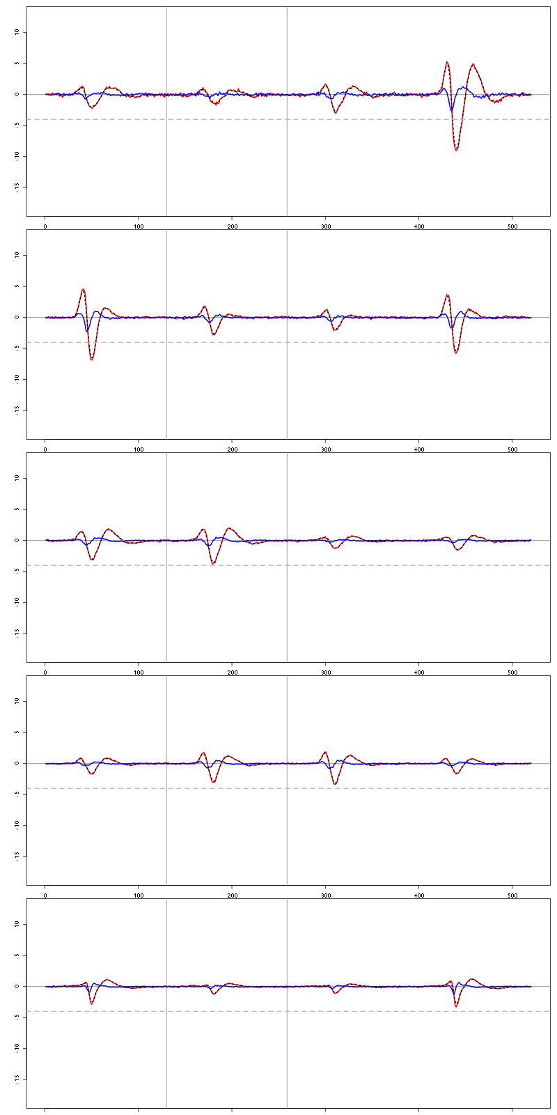
Figure 9: The last five templates (red) together with their first derivative (blue) all with the same scale. The dashed black curve show the templates filtered with the filter used during spike detection and the horizontal dashed grey line shows the detection threshold.

We see that the last three units won't reliably pass our threshold…

2.13 Peeling

We can now do the peeling.

2.13.1 Round 0

We classify, predict, subtract and check how many non-classified events we get:

round0 = lapply(as.vector(sp0),classify_and_align_evt,
                data=lD,centers=centers,
                before=c_before,after=c_after)
pred0 = predict_data(round0,centers,data_length = dim(lD)[1])
lD_1 = lD - pred0
sum(sapply(round0, function(l) l[[1]] == '?'))

We can see the difference before / after peeling for the data between 0.9 and 1.0 s:

ii = 1:1500 + 0.9*15000
tt = ii/15000
par(mar=c(1,1,1,1))
plot(tt, lD[ii,1], axes = FALSE,
     type="l",ylim=c(-100,20),
     xlab="",ylab="")
lines(tt, lD_1[ii,1], col='red')
lines(tt, lD[ii,2]-30, col='black')
lines(tt, lD_1[ii,2]-30, col='red')
lines(tt, lD[ii,3]-50, col='black')
lines(tt, lD_1[ii,3]-50, col='red')
lines(tt, lD[ii,4]-80, col='black')
lines(tt, lD_1[ii,4]-80, col='red')

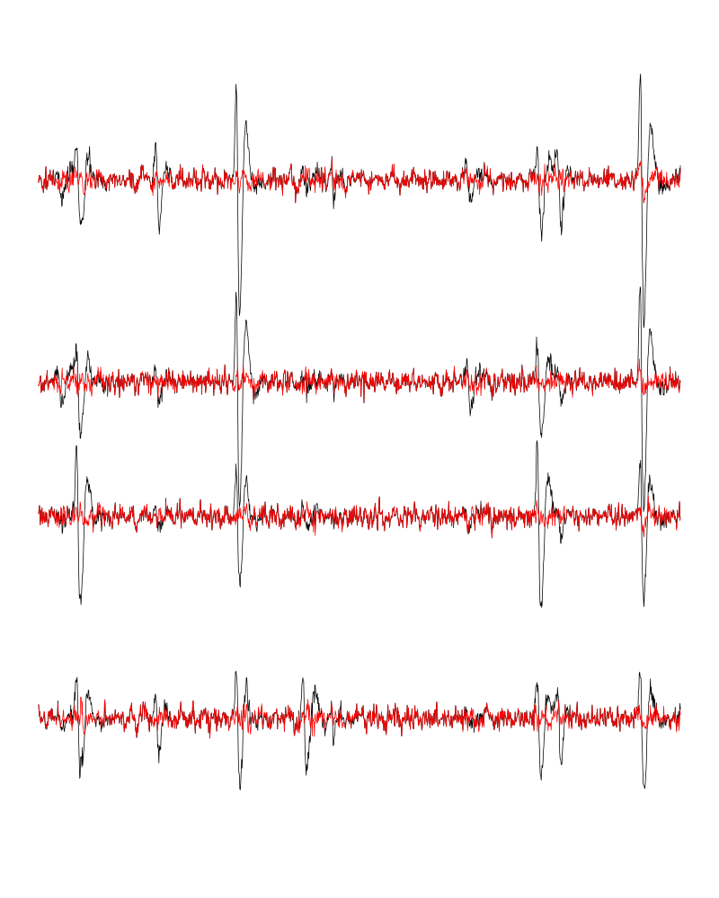
Figure 10: The first peeling illustrated on 100 ms of data, the raw data are in black and the first subtration in red.

2.13.2 Round 1

We keep going, using the subtracted data lD_1 as "raw data", detecting on all sites using the original MAD for normalization:

lDf = -lD_1
lDf = filter(lDf,rep(1,filter_length)/filter_length)
lDf[is.na(lDf)] = 0
lDf = t(t(lDf)/lDf_mad_original)
thrs = threshold_factor*c(1,1,1,1)
bellow.thrs = t(t(lDf) < thrs)
lDfr = lDf
lDfr[bellow.thrs] = 0
remove(lDf)
sp1 = peaks(apply(lDfr,1,sum),15)
remove(lDfr)
sp1

eventsPos object with indexes of 216 events. 
  Mean inter event interval: 1974.81 sampling points, corresponding SD: 2223.81 sampling points 
  Smallest and largest inter event intervals: 16 and 15982 sampling points.

We classify, predict, subtract and check how many non-classified events we get:

round1 = lapply(as.vector(sp1),classify_and_align_evt,
                data=lD_1,centers=centers,
                before=c_before,after=c_after)
pred1 = predict_data(round1,centers,data_length = dim(lD)[1])
lD_2 = lD_1 - pred1
sum(sapply(round1, function(l) l[[1]] == '?'))

We look at what's left with (not shown):

explore(sp1,lD_2,col=c("black","grey50"))

There is some stuff left but the big guys have disappeared so we decide to stop here.

2.14 Getting the spike trains

round_all = c(round0,round1)
spike_trains = lapply(paste("Cluster",1:nbc),
                      function(cn) sort(sapply(round_all[sapply(round_all,
                                                           function(l) l[[1]]==cn)],
                                          function(l) l[[2]]+l[[3]])))
names(spike_trains) = paste("Cluster",1:nbc)

2.15 Getting the inter spike intervals and the forward and backward recurrence times

2.15.1 ISI distributions

We first get the ISI (inter spike intervals) of each unit:

isi = sapply(spike_trains, diff)
names(isi) = names(spike_trains)

We define a plot_isi function that plots the ECDF (empirical cumulative distribution function) of the ISI:

plot_isi = function(isi, ## vector of ISIs
                    xlab="ISI (s)",
                    ylab="ECFD",
                    xlim=c(0,0.5), 
                    sampling_frequency=15000,
                    ... ## additional arguments passed to plot
                    ) {
    isi = sort(isi)/sampling_frequency
    n = length(isi)
    plot(isi,(1:n)/n,type="s",
         xlab=xlab,ylab=ylab,
         xlim=xlim,...)
}

We get the ISI ECDF for the units with:

layout(matrix(1:(nbc+nbc %% 2),nr=ceiling(nbc/2)))
par(mar=c(4,5,6,1))
for (cn in names(isi)) plot_isi(isi[[cn]],main=cn)

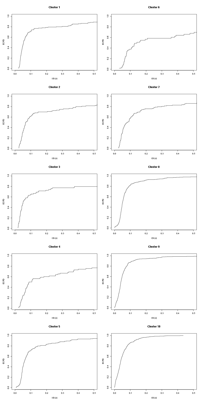
Figure 11: ISI ECDF for the ten units.

The first 7 look great the last three are clearly multi-unit.

2.15.2 Forward and Backward Recurrence Times

The forward recurrence time (FRT) between neuron A and B is the elapsed time between a spike in A and the next spike in B. The backward recurrence time (BRT) is the same thing except that we look for the former spike in B. If A and B are not correlated, the expected density of the FRT is the survival function (1-CDF) of the ISI from B divided by the mean ISI of B (the same holds for the BRT under the null hypothesis after taking the opposite). All that is correct if the data are stationary.

We define a function get_rt that returns the FRT and BRT given two spike trains:

get_rt = function(ref_train, 
                  test_train
                  ) {
    res=sapply(ref_train,
               function(t) c(max(test_train[test_train<=t])-t,
                             min(test_train[test_train>=t])-t)
               )
    res[,!apply(res,2,function(x) any(is.infinite(x)))]
}

We define next a function test_rt that plots a variance stabilized version of the histograms of the FRT and BRT minus the variance stabilized version under the null. The variance stabilization version is replacing the histogram bin counts $y$ by $\sqrt{y} + \sqrt{y+1}$. This transformation stabilizes the variance at 1.

test_rt = function(ref_train, 
                   test_train,
                   sampling_frequency=15000,
                   nbins=50, ## the number of breaks in the histogram
		   single_trial_duration = ceiling(max(c(ref_train,test_train))/sampling_frequency), 
                   xlab="Recurrence time (s)",
                   ylab="Stabilized counts - stabilized expected counts",
		   subdivisions = 10000, ## argument of integrate
                   ... ## additional parameters passed to plot
                   ) {
    rt = ref_train/sampling_frequency
    tt = test_train/sampling_frequency
    rt_L = vector("list",0)
    tt_L = vector("list",0)
    idx_max = max(c(rt,tt))%/%single_trial_duration
    if ( idx_max == 0) {
        rt_L = list(rt)
        tt_L = list(tt)
    } else {
        idx = 0
        while (idx <= idx_max) {
            start_trial_time = idx*single_trial_duration
            end_trial_time = start_trial_time + single_trial_duration
            rt_t = rt[start_trial_time <= rt & rt < end_trial_time]
            tt_t = tt[start_trial_time <= tt & tt < end_trial_time]
            if (length(rt_t) > 0 && length(tt_t) > 0) {
                rt_L = c(rt_L,list(rt_t-start_trial_time))
                tt_L = c(tt_L,list(tt_t-start_trial_time))
            }
            idx = idx + 1
        }
    }
    tt_isi_L = lapply(tt_L,diff)
    it = unlist(tt_isi_L)
    p_it=ecdf(it) ## ECDF of ISI from test
    mu_it=mean(it)
    s_it=function(t) (1-p_it(t))/mu_it ## expected density of FRT/BRT under the null
    ## Get the BRT and FRT
    res = lapply(1:length(rt_L),
                 function(idx) {
                     rt_t = rt_L[[idx]]
                     tt_t = tt_L[[idx]]
                     rt_t = rt_t[min(tt_t) < rt_t & rt_t < max(tt_t)]
                     RT = sapply(rt_t,
                                 function(t) c(max(tt_t[tt_t<=t])-t,
                                               min(tt_t[tt_t>=t])-t)
                                 )
                 })
    frt = sort(unlist(lapply(res, function(l) l[2,])))
    brt = sort(-unlist(lapply(res, function(l) l[1,])))
    n = length(frt)
    frt_h = hist(frt,breaks=nbins,plot=FALSE)
    frt_c_s = sqrt(frt_h$counts)+sqrt(frt_h$counts+1) ## stabilized version of the FRT counts
    ## expected FRT counts under the null
    frt_c_e = sapply(1:(length(frt_h$breaks)-1),
                     function(i) integrate(s_it,frt_h$breaks[i],frt_h$breaks[i+1],subdivisions = subdivisions)$value
                     )
    frt_c_e_s = sqrt(frt_c_e*n) + sqrt(frt_c_e*n+1) ## stabilized version of the expected FRT counts
    brt_h = hist(brt,breaks=nbins,plot=FALSE)
    brt_c_s = sqrt(brt_h$counts)+sqrt(brt_h$counts+1) ## stabilized version of the BRT counts
    ## expected BRT counts under the null
    brt_c_e = sapply(1:(length(brt_h$breaks)-1),
                     function(i) integrate(s_it,brt_h$breaks[i],brt_h$breaks[i+1],subdivisions = subdivisions)$value
                     )
    brt_c_e_s = sqrt(brt_c_e*n) + sqrt(brt_c_e*n+1) ## stabilized version of the expected BRT counts
    X = c(rev(-brt_h$mids),frt_h$mids)
    Y = c(rev(brt_c_s-brt_c_e_s),frt_c_s-frt_c_e_s)
    plot(X,Y,type="n",
         xlab=xlab,
         ylab=ylab,
         ...)
    abline(h=0,col="grey")
    abline(v=0,col="grey")
    lines(X,Y,type="s")
}

Notice that get_rt is included in test_rt so we don't really need the former anymore.

On the data at hand that gives for the first 7 units:

layout_matrix = matrix(0,nr=nbc-3,nc=nbc-3)
counter = 1
for (i in 1:(nbc-3))
    for (j in 1:(nbc-3))
        if (i != j) {
            layout_matrix[i,j] = counter
            counter = counter +1
        }
layout(layout_matrix)
par(mar=c(4,3,4,1))
for (i in 1:(nbc-3))
    for (j in 1:(nbc-3))
        if (i != j)
            test_rt(spike_trains[[i]],
                    spike_trains[[j]],
                    ylab="",main=paste("Units",i,"and",j))

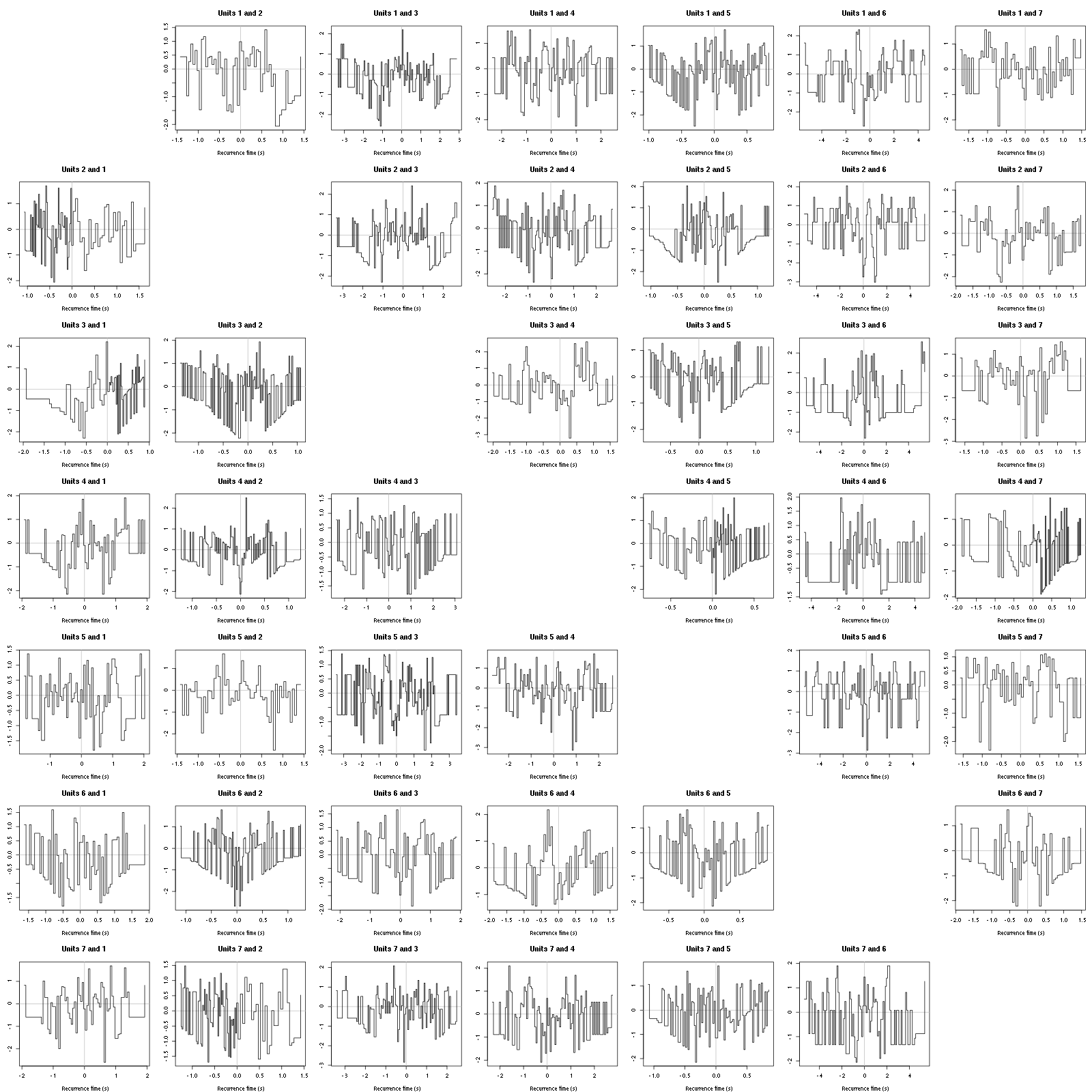
Figure 12: Graphical tests for the first 7 units of the Backward and Forward Reccurrence Times distrution agaisnt the null hypothesis (no interaction). If the null is correct, the curves should be IID draws from a standard normal distribution.

On this time scale with this number of events, we do not see signs of interactions.

2.16 Making "all at once"

Now that we have classified a single trial we would like to classify the subsequent ones (from the same experiment and the same tetrode) without re-estimating the model every time. If the recording conditions were perfectly stable we could proceed rather easily and in fact to the job in parallel. There are nevertheless few sources of variability we should be ready to cope with:

First and foremost we can observe a slow drift of the electrodes inducing a change in the relative positions of the neurons and the electrodes. This results in a change of the waveform generated by the neurons on the different recording sites. Since these drifts usually occur on a slow time scale (several minutes) the easiest way to deal with them is to process the data sequentially, in the order in which they were recorded (that precludes the parallel processing alluded to above) and to make the templates evolve slowly by computing, at the end of each trial a weighted average of the templates just used and of the ones obtained by averaging the well isolated events that were just classified.
A neuron can disappear (because it dies–don't forget that our probes are large and damage the neurons upon insertion–or because of the drift) or appear (because of the drift or "something else" like an hormonal regulation). In the latter case, the model (list of templates) should be updated to include a new element. In any case, the way to detect these appearances / disappearances is to monitor at the end of each trial classification the number of spikes attributed to each neuron of the model as well as the number of unclassified events.

2.16.1 What should our "all at once" function do?

The first thing is to print the five-number summary so that if something went really wrong (amplifier saturation, large noise increase) it will be readily detected. It is then a good idea to print after each peeling round the total number of detected events, the number of events attributed to each neuron and the number of unclassified events. At the end we want to print these same numbers obtained from the whole peeling procedure. The function will also return in a list the following elements:

prediction: A predicted trace (the overall version of the previous predX).
residual: A residual trace (the data minus the prediction).
classification: The round_all object above.
unknown: An events object containing the unclassified events (for quick monitoring in case of problems).
centers: A version of centers computed from the data just analyzed (so that the user can make a weighted average at will).
counts: A vector with the total number of events, the number of events from each neuron and the number of unclassified events.

Argument verbose controls the verbosity: if 0 nothing is printed to the stdout; if 1 the final results are printed; if 2 (default) the final and intermediate (following each peeling round) results are printed. A distinction is made between the first peeling round and the subsequent ones that can have different filter lengths (filter_length_1 and filter_length) and different minimalDist arguments for the peaks function that is called internally. The channels on which the detection is performed at each peeling round is controlled by the corresponding element of vector detection_cycle (a value 0 for an element means that the detection is performed on all channels).

2.16.2 `all_at_once` definition

So let us define our function:

all_at_once = function(data, ## an unormalized data matrix
                       centers, ## a list of centers
                       thres=4*c(1,1), ## threshold vector
                       filter_length_1=5, ## length of first filter
                       filter_length=5, ## length of subsequent filters
                       minimalDist_1=15, ## dead time length imposed at first detection
                       minimalDist=10, ## dead time length imposed at subsequent detection
                       before=c_before, ## parameter of centers
                       after=c_after, ## parameter of centers
                       detection_cycle=c(0,1,2,3,4), ## where is detection done during the peeling
                       verbose=2 ## verbosity level
                       ) {
    n_samples = dim(data)[1] ## Number of sample points
    n_chan = dim(data)[2] ## Number of channels
    n_rounds = length(detection_cycle)
    if (verbose > 0) {
        ## print five number summary
        cat("The five number summary is:\n")
        print(summary(data,digits=2))
        cat("\n")
    }
    ## normalize the data
    data.mad = apply(data,2,mad)
    data = t((t(data)-apply(data,2,median))/data.mad)
    filtered_data_mad = sapply(c(filter_length_1,filter_length),
                               function(l) {
                                   lDf = -data
                                   lDf = filter(lDf,rep(1,l)/l)
                                   lDf[is.na(lDf)] = 0
                                   apply(lDf,2,mad)
                               })
    ## Define local function detecting spikes
    get_sp = function(dataM,
                      f_length,
                      MAD,
                      site_idx=0,
                      minimalDist=15) {
        lDf = -dataM
        lDf = filter(lDf,rep(1,f_length)/f_length)
        lDf[is.na(lDf)] = 0
        lDf = t(t(lDf)/MAD)
        bellow.thrs = t(t(lDf) < thres)
        lDfr = lDf
        lDfr[bellow.thrs] = 0
        if (site_idx == 0)
            res = peaks(apply(lDfr,1,sum),minimalDist)
        else
            res = peaks(lDfr[,site_idx],minimalDist)
        res[res>before & res < dim(dataM)[1]-after]
    }
    
    out_names = c(names(centers),"?") ## Possible names for classification
    data0 = data ## The normalized version of the data
    for (r_idx in 1:n_rounds) {
        s_idx = detection_cycle[r_idx]
        if (verbose > 1 && s_idx==0)
            cat(paste("Doing now round",r_idx-1,"detecting on all sites\n"))
        if (verbose > 1 && s_idx!=0)
            cat(paste("Doing now round",r_idx-1,"detecting on site",s_idx,"\n"))
        sp = get_sp(dataM=data,
                    f_length=ifelse(r_idx==1,filter_length_1,filter_length),
                    MAD=filtered_data_mad[,ifelse(r_idx==1,1,2)],
                    site_idx=s_idx,
                    minimalDist=ifelse(r_idx==1,minimalDist_1,minimalDist))
        if (length(sp)==0) next
        new_round = lapply(as.vector(sp),classify_and_align_evt,
                           data=data,centers=centers,
                           before=before,after=after)
        pred = predict_data(new_round,centers,
                            nb_channels = n_chan,
                            data_length = n_samples)
        data = data - pred
        res = sapply(out_names,
                     function(n) sum(sapply(new_round, function(l) l[[1]] == n)))
        res = c(length(sp),res)
        names(res) = c("Total",out_names)
        if (verbose > 1) {
            print(res)
            cat("\n")
        }
        if (r_idx==1)
            round_all = new_round
        else
            round_all = c(round_all,new_round)
    }

    ## Get the global prediction
    pred = predict_data(round_all,centers,
                        nb_channels=n_chan,
                        data_length=n_samples)
    ## Get the residuals
    resid = data0 - pred
    ## Repeat inital detection on resid
    sp = get_sp(dataM=resid,
                f_length=filter_length_1,
		MAD=filtered_data_mad[,1],
                site_idx=detection_cycle[1],
                minimalDist=minimalDist_1)
    ## make events objects from this stuff
    unknown = mkEvents(sp,resid,before,after)
    ## get global counts
    res = sapply(out_names,
                 function(n) sum(sapply(round_all, function(l) l[[1]] == n)))
    res["?"] = length(sp)
    res=c(sum(res),res)
    names(res) = c("Total",out_names)
    if (verbose > 0) {
        cat("Global counts at classification's end:\n")
        print(res)
    }
    ## Get centers
    obs_nb = lapply(out_names[-length(out_names)],
                    function(cn) sum(sapply(round_all, function(l) l[[1]]==cn)))
    names(obs_nb) = out_names[-length(out_names)]
    spike_trains = lapply(out_names[-length(out_names)],
                          function(cn) {
                              if (obs_nb[cn] <= 1)
                                  return(numeric(0))
                              else
                                  res = sapply(round_all[sapply(round_all, function(l) l[[1]]==cn)],
                                               function(l)
                                                   round(l[[2]]+l[[3]]))
                              res[res>0 & res<n_samples]
                          }
                              )    
    centersN = lapply(1:length(spike_trains),
                      function(st_idx) {
                          if (length(spike_trains[[st_idx]]) == 0)
                              centers[[st_idx]]
                          else
                              mk_center_list(spike_trains[[st_idx]],data0,
                                             before=before,after=after)
                      }
                      )
    names(centersN) = out_names[-length(out_names)]
    list(prediction=pred,
         residual=resid,
         counts=res,
         unknown=unknown,
         centers=centersN,
         classification=round_all)
}

Argument verbose controls the level of "verbosity": if 0 nothing is printed to the stdout; if 1 the final results are printed; if 2 (default) the final and intermediate (following each peeling round) results are printed.

2.16.3 Test

We test the function with:

## We need again an un-normalized version of the data
ref_data = rbind(cbind(h5read("locust20010214_part1.hdf5", "/Spontaneous_2/trial_30/ch02"),
                       h5read("locust20010214_part1.hdf5", "/Spontaneous_2/trial_30/ch03"),
                       h5read("locust20010214_part1.hdf5", "/Spontaneous_2/trial_30/ch05"),
                       h5read("locust20010214_part1.hdf5", "/Spontaneous_2/trial_30/ch07")))
## We can now use our function
aao=all_at_once(data=ref_data, centers, thres=threshold_factor*c(1,1,1,1), 
                filter_length_1=filter_length, filter_length=filter_length, 
                minimalDist_1=15, minimalDist=15, 
                before=c_before, after=c_after, 
                detection_cycle=c(0,0), verbose=2)

The five number summary is:
       V1             V2             V3             V4      
 Min.   :  98   Min.   : 610   Min.   : 762   Min.   : 475  
 1st Qu.:2011   1st Qu.:2015   1st Qu.:2017   1st Qu.:2014  
 Median :2058   Median :2057   Median :2057   Median :2059  
 Mean   :2055   Mean   :2055   Mean   :2054   Mean   :2056  
 3rd Qu.:2105   3rd Qu.:2099   3rd Qu.:2095   3rd Qu.:2102  
 Max.   :3634   Max.   :3076   Max.   :2887   Max.   :3143  

Doing now round 0 detecting on all sites
     Total  Cluster 1  Cluster 2  Cluster 3  Cluster 4  Cluster 5  Cluster 6 
      1950        156        119         84         77        202         48 
 Cluster 7  Cluster 8  Cluster 9 Cluster 10          ? 
       126        285        401        433         19 

Doing now round 1 detecting on all sites
     Total  Cluster 1  Cluster 2  Cluster 3  Cluster 4  Cluster 5  Cluster 6 
       216          0          1          1          2          9          6 
 Cluster 7  Cluster 8  Cluster 9 Cluster 10          ? 
         3         44         51         78         21 

Global counts at classification's end:
     Total  Cluster 1  Cluster 2  Cluster 3  Cluster 4  Cluster 5  Cluster 6 
      2185        156        120         85         79        211         54 
 Cluster 7  Cluster 8  Cluster 9 Cluster 10          ? 
       129        329        452        511         59

We see that we are getting back the numbers we obtained before step by step.

We can compare the "old" and "new" centers with (not shown):

layout(matrix(1:nbc,nr=nbc))
par(mar=c(1,4,1,1))
for (i in 1:nbc) {
    plot(centers[[i]]$center,lwd=2,col=2,
         ylim=the_range,type="l")
    abline(h=0,col="grey50")
    abline(v=(c_before+c_after)+1,col="grey50")
    lines(aao$centers[[i]]$center,lwd=1,col=4)
}

They are not exactly identical since the new version is computed with all events (superposed or not) attributed to each neuron.

3 Analyzing a sequence of trials

3.1 Create a directory were results get saved

We will carry out an analysis of sequences of 30/25 trials with a given odor. At the end of the analysis of the sequence we will save some intermediate R object in a directory we are now creating.:

if (!dir.exists("tetB_analysis"))
    dir.create("tetB_analysis")

3.2 Create a data loading function

We want to write a function that takes a trial number and stimulus name and returns a matrix containing stereode Ca (channels 9, 11) data for this trial. The only little trick the function must include is the fact that a number x smaller than 10 appears in the data set name as 0x:

get_tetrode_data = function(trial_idx,stim="Spontaneous_1") {
    prefix = ifelse(trial_idx<10,
                    paste0("/",stim,"/trial_0",trial_idx),
                    paste0("/",stim,"/trial_",trial_idx)
                    )
    cbind(h5read("locust20010214_part1.hdf5", paste0(prefix,"/ch02")),
          h5read("locust20010214_part1.hdf5", paste0(prefix,"/ch03")),
          h5read("locust20010214_part1.hdf5", paste0(prefix,"/ch05")),
          h5read("locust20010214_part1.hdf5", paste0(prefix,"/ch07")))
}

3.3 `sort_many_trials` definition

We define now function sort_many_trials. This function takes the following formal parameters:

inter_trial_time: the time (in sample points) between two successive trials. Example 10*15000.
get_data_fct: a function loading the data of a single trial (like get_stereode_data we just defined). This function should take a trial number as its first argument and a sequence name as its second. Example get_stereode_data.
stim_name: the sequence name making the second argument of function get_data_fct. Example "1-Hexanol".
trial_nbs: a vector containing the indices of the trials to sort. Example 1:30.
centers: a list like the centers list above. Example aao$centers.
counts: a vector with the number of counts each unit got at the previous stage. Example aao$counts.
all_at_once_call_list: a named list with the arguments used in the previous call to all at once except the first two.
layout_matrix: a matrix controlling the layout of the diagnostic plots generated while the function is running.
new_weight_in_update: the maximal weight of the new template in the estimation of the current one.

The function returns a list with the following elements:

centers: the last estimation of the templates.
counts: the last counts.
centers_L: a list of matrices. Each matrix contains the successive template for each neuron (used to track template evolution).
counts_M: a matrix with the successive counts.
spike_trains: a list of spike trains, one per neuron.

sort_many_trials = function(inter_trial_time,
                            get_data_fct,
                            stim_name,
                            trial_nbs,
                            centers,
                            counts,
                            all_at_once_call_list=list(thres=4*c(1,1), 
                                                       filter_length_1=5, filter_length=3, 
                                                       minimalDist_1=15, minimalDist=10, 
                                                       before=c_before, after=c_after, 
                                                       detection_cycle=c(0,0), verbose=1),
                            layout_matrix=matrix(1:10,nr=5),
                            new_weight_in_update=0.01
                            ) {
    centers_old = centers
    counts_old = counts
    counts_M = matrix(0,nr=length(trial_nbs),nc=length(counts_old))
    centers_L = lapply(centers,
                       function(c) {
                           res = matrix(0,nr=length(c$center),nc=length(trial_nbs))
                           res[,1] = c$center
                           res
                       }
                       )
    names(centers_L) = names(centers)
    nbc = length(centers)
    spike_trains = vector("list",nbc)
    names(spike_trains) = paste("Cluster",1:nbc)
    idx=1
    for (trial_idx in trial_nbs) {
        ref_data = get_data_fct(trial_idx,stim_name)
        cat(paste0("***************\nDoing now trial ",trial_idx," of ",stim_name,"\n"))
        analysis = do.call(all_at_once,
                           c(list(data=ref_data,centers=centers),all_at_once_call_list))
        cat(paste0("Trial ",trial_idx," done!\n******************\n"))
        centers_new = analysis$centers
        counts_new = analysis$counts
        counts_M[idx,] = counts_new
        centers = centers_new
        for (c_idx in 1:length(centers)){
            n = counts_new[c_idx+1]
            o = counts_old[c_idx+1]
            w = new_weight_in_update*ifelse(o>0,min(1,n/o),0) ## New template weight
            centers[[c_idx]]$center=w*centers_new[[c_idx]]$center+(1-w)*centers_old[[c_idx]]$center
            centers[[c_idx]]$centerD=w*centers_new[[c_idx]]$centerD+(1-w)*centers_old[[c_idx]]$centerD
            centers[[c_idx]]$centerDD=w*centers_new[[c_idx]]$centerDD+(1-w)*centers_old[[c_idx]]$centerDD
            centers[[c_idx]]$centerD_norm2=sum(centers[[c_idx]]$centerD^2)
            centers[[c_idx]]$centerDD_norm2=sum(centers[[c_idx]]$centerDD^2)
            centers[[c_idx]]$centerD_dot_centerDD=sum(centers[[c_idx]]$centerD*centers[[c_idx]]$centerDD)
            centers_L[[c_idx]][,idx] = centers[[c_idx]]$center
        }
        layout(layout_matrix)
        par(mar=c(1,3,3,1))
        the_pch = if (nbc<10) c(paste(1:nbc),"?")
                  else c(paste(1:9),letters[1:(nbc-9)],"?")
        matplot(counts_M[,2:length(counts_old)],type="b",
                pch=the_pch)
        c_range = range(sapply(centers_L,
                               function(m) range(m[,1:idx])))
        for (i in 1:nbc) {
            if (idx<3)
                matplot(centers_L[[i]][,1:idx],type="l",col=1,lty=1,lwd=0.5,
                        main=paste("Unit",i),ylim=c_range)
            else
                matplot(centers_L[[i]][,1:idx],type="l",col=c(4,rep(1,idx-2),2),
                        lty=1,lwd=0.5,main=paste("Unit",i),ylim=c_range)
        }
        centers_old = centers
        counts_old = counts_new
        round_all = analysis$classification
        st = lapply(paste("Cluster",1:nbc),
                    function(cn) sapply(round_all[sapply(round_all,
                                                         function(l) l[[1]]==cn)],
                                        function(l) l[[2]]+l[[3]]))
        names(st) = paste("Cluster",1:nbc)
        for (cn in paste("Cluster",1:nbc)) {
            if (length(st[[cn]]) > 0)
                spike_trains[[cn]] = c(spike_trains[[cn]],
                (trial_idx-1)*inter_trial_time + sort(st[[cn]]))
        }
        idx = idx+1
    }
    spike_trains = lapply(spike_trains,sort)
    list(centers=centers,
         counts=counts_new,
         spike_trains=spike_trains,
         counts_M=counts_M,
         centers_L=centers_L,
         trial_nbs=trial_nbs,
	 call=match.call())
}

3.4 Diagnostic plot function definitions

We define next three functions defining diagnostic plots at the end of a sequence analysis:

counts_evolution = function(smt_res ## result of a sort_many_trials call
                           ) {
    nbc = length(smt_res$centers)
    the_pch = if (nbc<10) c(paste(1:nbc),"?")
                  else c(paste(1:9),letters[1:(nbc-9)],"?")
    matplot(smt_res$trial_nbs,
            smt_res$counts_M[,2:(nbc+2)],
            type="b",pch=the_pch,
            main="Counts evolution",xlab="Trial index",ylab="Number of events")
}

waveform_evolution = function(smt_res, ## result of a sort_many_trials call
                              threshold_factor=4, ## threshold used
                              layout_matrix=matrix(1:nbc,nr=nbc)
                              ) {
    nbc = length(smt_res$centers)
    nt = length(smt_res$trial_nbs)
    layout(layout_matrix)
    par(mar=c(1,3,4,1))
    for (i in 1:nbc) {
        matplot(smt_res$centers_L[[i]],
                type="l",col=c(4,rep(1,nt-2),2),lty=1,lwd=0.5,
                main=paste("Unit",i),ylab="")
        abline(h=-threshold_factor,col="grey")
        }
}

cp_isi=function(smt_res, ## result of a sort_many_trials call
                inter_trial_time=10, ## time between trials in seconds
                sampling_rate=15000, ## sampling rate in Hz
                nbins=50, ## number of bins for isi histogram
                isi_max=1, ## largest isi in isi histogram
                layout_matrix=matrix(1:(2*still_there),nr=still_there,byrow=TRUE)
                ) {
    t_duration = inter_trial_time
    n_trials = length(smt_res$trial_nbs)
    nbc = length(smt_res$centers)
    still_there = nbc - sum(sapply(smt_res$spike_trains,
                                   function(l)
                                       is.null(l) || length(l) <= n_trials))
    layout(layout_matrix)
    par(mar=c(4,4,4,1))
    for (cn in names(smt_res$spike_trains)) {
        if (is.null(smt_res$spike_trains[[cn]]) || length(smt_res$spike_trains[[cn]]) <= n_trials) next
        st = smt_res$spike_trains[[cn]]/sampling_rate
        plot(st,1:length(st),
             main=paste("Observed CP for unit",cn),
             xlab="Time (s)",ylab="Nb of evts",type="s")
        isi = diff(st)
        isi = isi[isi <= isi_max]
        hist(isi,breaks=nbins,
             prob=TRUE,xlim=c(0,0.5),
             main=paste("ISI dist for unit",cn),
             xlab="Interval (s)",ylab="Density (1/s)")
    } 
}

cp_isi_raster=function(smt_res, ## result of a sort_many_trials call
                      inter_trial_time=10, ## time between trials in seconds
                      sampling_rate=15000, ## sampling rate in Hz
                      nbins=50, ## number of bins for isi histogram
                      isi_max=1, ## largest isi in isi histogram
                      layout_matrix=matrix(1:(3*still_there),nr=still_there,byrow=TRUE)
                      ) {
    t_duration = inter_trial_time
    n_trials = length(smt_res$trial_nbs)
    nbc = length(smt_res$centers)
    still_there = nbc - sum(sapply(smt_res$spike_trains,
                                   function(l)
                                       is.null(l) || length(l) <= n_trials))
    layout(layout_matrix)
    par(mar=c(4,4,4,1))
    for (cn in names(smt_res$spike_trains)) {
        if (is.null(smt_res$spike_trains[[cn]]) || length(smt_res$spike_trains[[cn]]) <= n_trials) next
        st = smt_res$spike_trains[[cn]]/sampling_rate
        plot(st,1:length(st),
             main=paste("Observed CP for unit",cn),
             xlab="Time (s)",ylab="Nb of evts",type="s")
        isi = diff(st)
        isi = isi[isi <= isi_max]
        hist(isi,breaks=nbins,
             prob=TRUE,xlim=c(0,0.5),
             main=paste("ISI dist for unit",cn),
             xlab="Interval (s)",ylab="Density (1/s)")
        plot(c(0,t_duration),c(0,n_trials+1),type="n",axes=FALSE,
             xlab="",ylab="",main=paste("Raster of unit",cn))
        for (t_idx in 1:n_trials) {
            sub_st = st[(t_idx-1)*t_duration <= st &
                        st < t_idx*t_duration] - (t_idx-1)*t_duration
            if (length(sub_st) > 0)
                points(sub_st, rep(t_idx,length(sub_st)), pch=".")
        }
    } 
}

4 Systematic analysis of the 30 trials from `Spontaneous_2` backwards

We will carry out an analysis of the 30 trials of Spontaenous_2 backwards since the model was estimated from the last trial. The LabBook mentions that that noise is present at trials 23, 24 and 25 so we skip these trials.

4.1 Doing the job

a_Spontaneous_2_tetB=sort_many_trials(inter_trial_time=30*15000,
                                      get_data_fct=get_tetrode_data,
                                      stim_name="Spontaneous_2",
                                      trial_nbs=rev(c(1:22,26:30)),
                                      centers=aao$centers,
                                      counts=aao$counts,
                                      all_at_once_call_list=list(thres=threshold_factor*c(1,1,1,1), 
                                                                 filter_length_1=filter_length, filter_length=filter_length, 
                                                                 minimalDist_1=15, minimalDist=15, 
                                                                 before=c_before, after=c_after, 
                                                                 detection_cycle=c(0,0), verbose=1),
                                      layout_matrix=matrix(c(1,1:11),nr=6),new_weight_in_update=0.01
                                      )

***************
Doing now trial 30 of Spontaneous_2
The five number summary is:
       V1             V2             V3             V4      
 Min.   :  98   Min.   : 610   Min.   : 762   Min.   : 475  
 1st Qu.:2011   1st Qu.:2015   1st Qu.:2017   1st Qu.:2014  
 Median :2058   Median :2057   Median :2057   Median :2059  
 Mean   :2055   Mean   :2055   Mean   :2054   Mean   :2056  
 3rd Qu.:2105   3rd Qu.:2099   3rd Qu.:2095   3rd Qu.:2102  
 Max.   :3634   Max.   :3076   Max.   :2887   Max.   :3143  

Global counts at classification's end:
     Total  Cluster 1  Cluster 2  Cluster 3  Cluster 4  Cluster 5  Cluster 6 
      2193        156        120         85         78        208         53 
 Cluster 7  Cluster 8  Cluster 9 Cluster 10          ? 
       130        337        447        517         62 
Trial 30 done!
******************
***************
Doing now trial 29 of Spontaneous_2
The five number summary is:
       V1             V2             V3             V4      
 Min.   : 229   Min.   : 663   Min.   :1029   Min.   : 786  
 1st Qu.:2010   1st Qu.:2014   1st Qu.:2017   1st Qu.:2014  
 Median :2058   Median :2057   Median :2057   Median :2059  
 Mean   :2055   Mean   :2055   Mean   :2054   Mean   :2056  
 3rd Qu.:2105   3rd Qu.:2099   3rd Qu.:2095   3rd Qu.:2102  
 Max.   :3339   Max.   :3083   Max.   :2755   Max.   :3033  

Global counts at classification's end:
     Total  Cluster 1  Cluster 2  Cluster 3  Cluster 4  Cluster 5  Cluster 6 
      2220        118        119         51        143        232         38 
 Cluster 7  Cluster 8  Cluster 9 Cluster 10          ? 
       154        350        349        570         96 
Trial 29 done!
******************
***************
Doing now trial 28 of Spontaneous_2
The five number summary is:
       V1             V2             V3             V4      
 Min.   : 265   Min.   : 652   Min.   : 960   Min.   : 889  
 1st Qu.:2011   1st Qu.:2014   1st Qu.:2017   1st Qu.:2014  
 Median :2058   Median :2057   Median :2057   Median :2059  
 Mean   :2055   Mean   :2055   Mean   :2054   Mean   :2056  
 3rd Qu.:2105   3rd Qu.:2099   3rd Qu.:2095   3rd Qu.:2102  
 Max.   :3260   Max.   :3137   Max.   :2837   Max.   :2871  

Global counts at classification's end:
     Total  Cluster 1  Cluster 2  Cluster 3  Cluster 4  Cluster 5  Cluster 6 
      2100        110        164         42        124        284         63 
 Cluster 7  Cluster 8  Cluster 9 Cluster 10          ? 
       137        300        306        493         77 
Trial 28 done!
******************
***************
Doing now trial 27 of Spontaneous_2
The five number summary is:
       V1             V2             V3             V4      
 Min.   : 412   Min.   : 533   Min.   :1025   Min.   : 742  
 1st Qu.:2012   1st Qu.:2015   1st Qu.:2018   1st Qu.:2015  
 Median :2058   Median :2057   Median :2057   Median :2058  
 Mean   :2056   Mean   :2055   Mean   :2055   Mean   :2056  
 3rd Qu.:2104   3rd Qu.:2099   3rd Qu.:2094   3rd Qu.:2101  
 Max.   :3304   Max.   :3133   Max.   :2742   Max.   :3102  

Global counts at classification's end:
     Total  Cluster 1  Cluster 2  Cluster 3  Cluster 4  Cluster 5  Cluster 6 
      2038        120        123         58         60        231         23 
 Cluster 7  Cluster 8  Cluster 9 Cluster 10          ? 
       146        366        368        466         77 
Trial 27 done!
******************
***************
Doing now trial 26 of Spontaneous_2
The five number summary is:
       V1             V2             V3             V4      
 Min.   : 442   Min.   : 715   Min.   : 988   Min.   : 789  
 1st Qu.:2012   1st Qu.:2015   1st Qu.:2017   1st Qu.:2014  
 Median :2058   Median :2057   Median :2057   Median :2058  
 Mean   :2056   Mean   :2055   Mean   :2054   Mean   :2056  
 3rd Qu.:2104   3rd Qu.:2098   3rd Qu.:2094   3rd Qu.:2101  
 Max.   :3263   Max.   :3140   Max.   :2924   Max.   :3014  

Global counts at classification's end:
     Total  Cluster 1  Cluster 2  Cluster 3  Cluster 4  Cluster 5  Cluster 6 
      2024         92        111         56        123        176         33 
 Cluster 7  Cluster 8  Cluster 9 Cluster 10          ? 
       160        240        414        543         76 
Trial 26 done!
******************
***************
Doing now trial 22 of Spontaneous_2
The five number summary is:
       V1             V2             V3             V4      
 Min.   : 287   Min.   : 529   Min.   : 656   Min.   : 795  
 1st Qu.:2012   1st Qu.:2015   1st Qu.:2018   1st Qu.:2015  
 Median :2058   Median :2057   Median :2057   Median :2059  
 Mean   :2056   Mean   :2055   Mean   :2054   Mean   :2056  
 3rd Qu.:2103   3rd Qu.:2098   3rd Qu.:2094   3rd Qu.:2101  
 Max.   :3253   Max.   :3077   Max.   :3046   Max.   :3202  

Global counts at classification's end:
     Total  Cluster 1  Cluster 2  Cluster 3  Cluster 4  Cluster 5  Cluster 6 
      1942        111        140         59        116        202         23 
 Cluster 7  Cluster 8  Cluster 9 Cluster 10          ? 
       123        289        325        476         78 
Trial 22 done!
******************
***************
Doing now trial 21 of Spontaneous_2
The five number summary is:
       V1             V2             V3             V4      
 Min.   : 141   Min.   : 642   Min.   :1081   Min.   : 937  
 1st Qu.:2011   1st Qu.:2015   1st Qu.:2017   1st Qu.:2014  
 Median :2058   Median :2057   Median :2056   Median :2059  
 Mean   :2056   Mean   :2055   Mean   :2054   Mean   :2056  
 3rd Qu.:2104   3rd Qu.:2099   3rd Qu.:2094   3rd Qu.:2102  
 Max.   :3474   Max.   :3006   Max.   :2838   Max.   :3148  

Global counts at classification's end:
     Total  Cluster 1  Cluster 2  Cluster 3  Cluster 4  Cluster 5  Cluster 6 
      1914        128        107         65        122        246         29 
 Cluster 7  Cluster 8  Cluster 9 Cluster 10          ? 
       115        283        282        451         86 
Trial 21 done!
******************
***************
Doing now trial 20 of Spontaneous_2
The five number summary is:
       V1             V2             V3             V4      
 Min.   : 343   Min.   : 645   Min.   : 830   Min.   : 834  
 1st Qu.:2012   1st Qu.:2015   1st Qu.:2017   1st Qu.:2014  
 Median :2058   Median :2057   Median :2056   Median :2059  
 Mean   :2055   Mean   :2055   Mean   :2054   Mean   :2056  
 3rd Qu.:2104   3rd Qu.:2099   3rd Qu.:2094   3rd Qu.:2102  
 Max.   :3295   Max.   :3059   Max.   :2915   Max.   :2951  

Global counts at classification's end:
     Total  Cluster 1  Cluster 2  Cluster 3  Cluster 4  Cluster 5  Cluster 6 
      2004        172        112         79         72        232         42 
 Cluster 7  Cluster 8  Cluster 9 Cluster 10          ? 
       151        348        220        475        101 
Trial 20 done!
******************
***************
Doing now trial 19 of Spontaneous_2
The five number summary is:
       V1             V2             V3             V4      
 Min.   : 527   Min.   : 642   Min.   : 830   Min.   : 796  
 1st Qu.:2011   1st Qu.:2015   1st Qu.:2017   1st Qu.:2014  
 Median :2058   Median :2057   Median :2057   Median :2059  
 Mean   :2055   Mean   :2055   Mean   :2054   Mean   :2056  
 3rd Qu.:2105   3rd Qu.:2099   3rd Qu.:2094   3rd Qu.:2102  
 Max.   :3199   Max.   :3136   Max.   :2914   Max.   :3006  

Global counts at classification's end:
     Total  Cluster 1  Cluster 2  Cluster 3  Cluster 4  Cluster 5  Cluster 6 
      2117        135        138         23        144        193         24 
 Cluster 7  Cluster 8  Cluster 9 Cluster 10          ? 
       180        299        309        562        110 
Trial 19 done!
******************
***************
Doing now trial 18 of Spontaneous_2
The five number summary is:
       V1             V2             V3             V4      
 Min.   : 449   Min.   : 617   Min.   : 800   Min.   : 825  
 1st Qu.:2012   1st Qu.:2015   1st Qu.:2018   1st Qu.:2015  
 Median :2058   Median :2057   Median :2057   Median :2059  
 Mean   :2055   Mean   :2055   Mean   :2054   Mean   :2056  
 3rd Qu.:2104   3rd Qu.:2098   3rd Qu.:2095   3rd Qu.:2102  
 Max.   :3136   Max.   :2970   Max.   :2887   Max.   :2921  

Global counts at classification's end:
     Total  Cluster 1  Cluster 2  Cluster 3  Cluster 4  Cluster 5  Cluster 6 
      2050        138        145         69         65        215         37 
 Cluster 7  Cluster 8  Cluster 9 Cluster 10          ? 
       134        282        372        519         74 
Trial 18 done!
******************
***************
Doing now trial 17 of Spontaneous_2
The five number summary is:
       V1             V2             V3             V4      
 Min.   : 270   Min.   : 580   Min.   :1061   Min.   : 598  
 1st Qu.:2012   1st Qu.:2015   1st Qu.:2017   1st Qu.:2015  
 Median :2058   Median :2057   Median :2057   Median :2059  
 Mean   :2056   Mean   :2055   Mean   :2054   Mean   :2056  
 3rd Qu.:2104   3rd Qu.:2099   3rd Qu.:2094   3rd Qu.:2101  
 Max.   :3323   Max.   :3047   Max.   :2830   Max.   :3172  

Global counts at classification's end:
     Total  Cluster 1  Cluster 2  Cluster 3  Cluster 4  Cluster 5  Cluster 6 
      2109        139        134         71        132        204         42 
 Cluster 7  Cluster 8  Cluster 9 Cluster 10          ? 
       116        255        441        479         96 
Trial 17 done!
******************
***************
Doing now trial 16 of Spontaneous_2
The five number summary is:
       V1             V2             V3             V4      
 Min.   : 397   Min.   : 600   Min.   : 818   Min.   : 684  
 1st Qu.:2011   1st Qu.:2015   1st Qu.:2017   1st Qu.:2014  
 Median :2058   Median :2057   Median :2057   Median :2059  
 Mean   :2055   Mean   :2055   Mean   :2054   Mean   :2056  
 3rd Qu.:2105   3rd Qu.:2099   3rd Qu.:2095   3rd Qu.:2102  
 Max.   :3343   Max.   :3116   Max.   :2995   Max.   :3070  

Global counts at classification's end:
     Total  Cluster 1  Cluster 2  Cluster 3  Cluster 4  Cluster 5  Cluster 6 
      2149        143        136         78        123        236         61 
 Cluster 7  Cluster 8  Cluster 9 Cluster 10          ? 
       153        302        312        512         93 
Trial 16 done!
******************
***************
Doing now trial 15 of Spontaneous_2
The five number summary is:
       V1             V2             V3             V4      
 Min.   : 392   Min.   : 691   Min.   : 763   Min.   : 736  
 1st Qu.:2012   1st Qu.:2016   1st Qu.:2018   1st Qu.:2015  
 Median :2058   Median :2057   Median :2056   Median :2058  
 Mean   :2056   Mean   :2055   Mean   :2054   Mean   :2056  
 3rd Qu.:2103   3rd Qu.:2098   3rd Qu.:2094   3rd Qu.:2101  
 Max.   :3264   Max.   :2989   Max.   :2960   Max.   :2984  

Global counts at classification's end:
     Total  Cluster 1  Cluster 2  Cluster 3  Cluster 4  Cluster 5  Cluster 6 
      1901        118        132         49         90        178         30 
 Cluster 7  Cluster 8  Cluster 9 Cluster 10          ? 
       144        280        360        432         88 
Trial 15 done!
******************
***************
Doing now trial 14 of Spontaneous_2
The five number summary is:
       V1             V2             V3             V4      
 Min.   : 270   Min.   : 592   Min.   :1018   Min.   : 604  
 1st Qu.:2012   1st Qu.:2016   1st Qu.:2017   1st Qu.:2015  
 Median :2058   Median :2057   Median :2057   Median :2059  
 Mean   :2056   Mean   :2055   Mean   :2054   Mean   :2056  
 3rd Qu.:2104   3rd Qu.:2098   3rd Qu.:2095   3rd Qu.:2101  
 Max.   :3213   Max.   :3061   Max.   :2801   Max.   :3016  

Global counts at classification's end:
     Total  Cluster 1  Cluster 2  Cluster 3  Cluster 4  Cluster 5  Cluster 6 
      1959        135        109         66         69        216         21 
 Cluster 7  Cluster 8  Cluster 9 Cluster 10          ? 
       105        231        441        498         68 
Trial 14 done!
******************
***************
Doing now trial 13 of Spontaneous_2
The five number summary is:
       V1             V2             V3             V4      
 Min.   :   0   Min.   :   0   Min.   :  24   Min.   :  78  
 1st Qu.:2011   1st Qu.:2015   1st Qu.:2017   1st Qu.:2014  
 Median :2058   Median :2058   Median :2057   Median :2059  
 Mean   :2055   Mean   :2055   Mean   :2054   Mean   :2056  
 3rd Qu.:2105   3rd Qu.:2100   3rd Qu.:2095   3rd Qu.:2102  
 Max.   :4073   Max.   :4073   Max.   :4073   Max.   :4072  

Global counts at classification's end:
     Total  Cluster 1  Cluster 2  Cluster 3  Cluster 4  Cluster 5  Cluster 6 
      2098        110        133         88         66        244         39 
 Cluster 7  Cluster 8  Cluster 9 Cluster 10          ? 
       151        318        382        465        102 
Trial 13 done!
******************
***************
Doing now trial 12 of Spontaneous_2
The five number summary is:
       V1             V2             V3             V4      
 Min.   : 133   Min.   : 487   Min.   : 785   Min.   : 487  
 1st Qu.:2012   1st Qu.:2015   1st Qu.:2017   1st Qu.:2015  
 Median :2058   Median :2057   Median :2057   Median :2058  
 Mean   :2056   Mean   :2055   Mean   :2055   Mean   :2056  
 3rd Qu.:2103   3rd Qu.:2098   3rd Qu.:2094   3rd Qu.:2101  
 Max.   :3344   Max.   :2981   Max.   :2864   Max.   :3228  

Global counts at classification's end:
     Total  Cluster 1  Cluster 2  Cluster 3  Cluster 4  Cluster 5  Cluster 6 
      2050        141        112         58         62        208         28 
 Cluster 7  Cluster 8  Cluster 9 Cluster 10          ? 
       117        258        335        587        144 
Trial 12 done!
******************
***************
Doing now trial 11 of Spontaneous_2
The five number summary is:
       V1             V2             V3             V4      
 Min.   : 197   Min.   : 522   Min.   : 720   Min.   : 632  
 1st Qu.:2012   1st Qu.:2015   1st Qu.:2017   1st Qu.:2015  
 Median :2058   Median :2057   Median :2057   Median :2058  
 Mean   :2056   Mean   :2055   Mean   :2054   Mean   :2056  
 3rd Qu.:2103   3rd Qu.:2098   3rd Qu.:2094   3rd Qu.:2101  
 Max.   :3292   Max.   :3067   Max.   :2885   Max.   :3102  

Global counts at classification's end:
     Total  Cluster 1  Cluster 2  Cluster 3  Cluster 4  Cluster 5  Cluster 6 
      1963        114        112         74         85        193         37 
 Cluster 7  Cluster 8  Cluster 9 Cluster 10          ? 
       127        259        303        526        133 
Trial 11 done!
******************
***************
Doing now trial 10 of Spontaneous_2
The five number summary is:
       V1             V2             V3             V4      
 Min.   : 314   Min.   : 715   Min.   : 924   Min.   : 797  
 1st Qu.:2011   1st Qu.:2014   1st Qu.:2017   1st Qu.:2014  
 Median :2058   Median :2057   Median :2056   Median :2058  
 Mean   :2055   Mean   :2055   Mean   :2054   Mean   :2056  
 3rd Qu.:2104   3rd Qu.:2099   3rd Qu.:2095   3rd Qu.:2102  
 Max.   :3434   Max.   :3140   Max.   :2998   Max.   :3197  

Global counts at classification's end:
     Total  Cluster 1  Cluster 2  Cluster 3  Cluster 4  Cluster 5  Cluster 6 
      2022        144        152         64        110        222         37 
 Cluster 7  Cluster 8  Cluster 9 Cluster 10          ? 
       150        280        324        438        101 
Trial 10 done!
******************
***************
Doing now trial 9 of Spontaneous_2
The five number summary is:
       V1             V2             V3             V4      
 Min.   : 332   Min.   : 669   Min.   :1046   Min.   : 721  
 1st Qu.:2012   1st Qu.:2015   1st Qu.:2017   1st Qu.:2014  
 Median :2058   Median :2057   Median :2057   Median :2058  
 Mean   :2056   Mean   :2055   Mean   :2054   Mean   :2056  
 3rd Qu.:2103   3rd Qu.:2098   3rd Qu.:2095   3rd Qu.:2101  
 Max.   :3206   Max.   :2984   Max.   :2869   Max.   :3094  

Global counts at classification's end:
     Total  Cluster 1  Cluster 2  Cluster 3  Cluster 4  Cluster 5  Cluster 6 
      1995         94        152         66         98        208         49 
 Cluster 7  Cluster 8  Cluster 9 Cluster 10          ? 
       145        210        381        462        130 
Trial 9 done!
******************
***************
Doing now trial 8 of Spontaneous_2
The five number summary is:
       V1             V2             V3             V4      
 Min.   : 103   Min.   : 415   Min.   : 887   Min.   : 572  
 1st Qu.:2012   1st Qu.:2015   1st Qu.:2017   1st Qu.:2015  
 Median :2058   Median :2057   Median :2057   Median :2058  
 Mean   :2056   Mean   :2055   Mean   :2054   Mean   :2056  
 3rd Qu.:2103   3rd Qu.:2098   3rd Qu.:2095   3rd Qu.:2101  
 Max.   :3433   Max.   :3069   Max.   :2863   Max.   :3104  

Global counts at classification's end:
     Total  Cluster 1  Cluster 2  Cluster 3  Cluster 4  Cluster 5  Cluster 6 
      1903        110        111         66         68        177         24 
 Cluster 7  Cluster 8  Cluster 9 Cluster 10          ? 
       141        233        437        433        103 
Trial 8 done!
******************
***************
Doing now trial 7 of Spontaneous_2
The five number summary is:
       V1             V2             V3             V4      
 Min.   : 151   Min.   : 613   Min.   : 769   Min.   : 670  
 1st Qu.:2011   1st Qu.:2014   1st Qu.:2017   1st Qu.:2014  
 Median :2059   Median :2057   Median :2057   Median :2059  
 Mean   :2055   Mean   :2055   Mean   :2054   Mean   :2056  
 3rd Qu.:2105   3rd Qu.:2100   3rd Qu.:2096   3rd Qu.:2102  
 Max.   :3575   Max.   :3074   Max.   :3080   Max.   :3132  

Global counts at classification's end:
     Total  Cluster 1  Cluster 2  Cluster 3  Cluster 4  Cluster 5  Cluster 6 
      2161        174        138         76         92        272         18 
 Cluster 7  Cluster 8  Cluster 9 Cluster 10          ? 
       157        349        304        458        123 
Trial 7 done!
******************
***************
Doing now trial 6 of Spontaneous_2
The five number summary is:
       V1             V2             V3             V4      
 Min.   : 263   Min.   : 680   Min.   : 932   Min.   : 472  
 1st Qu.:2011   1st Qu.:2014   1st Qu.:2016   1st Qu.:2014  
 Median :2058   Median :2057   Median :2057   Median :2059  
 Mean   :2055   Mean   :2055   Mean   :2054   Mean   :2056  
 3rd Qu.:2105   3rd Qu.:2100   3rd Qu.:2096   3rd Qu.:2102  
 Max.   :3283   Max.   :2953   Max.   :2937   Max.   :3205  

Global counts at classification's end:
     Total  Cluster 1  Cluster 2  Cluster 3  Cluster 4  Cluster 5  Cluster 6 
      2091        159        143         90        101        234         18 
 Cluster 7  Cluster 8  Cluster 9 Cluster 10          ? 
       138        301        375        425        107 
Trial 6 done!
******************
***************
Doing now trial 5 of Spontaneous_2
The five number summary is:
       V1             V2             V3             V4      
 Min.   : 334   Min.   : 737   Min.   : 956   Min.   : 478  
 1st Qu.:2011   1st Qu.:2014   1st Qu.:2017   1st Qu.:2014  
 Median :2058   Median :2057   Median :2057   Median :2059  
 Mean   :2055   Mean   :2055   Mean   :2054   Mean   :2056  
 3rd Qu.:2104   3rd Qu.:2099   3rd Qu.:2095   3rd Qu.:2102  
 Max.   :3238   Max.   :2998   Max.   :2817   Max.   :3235  

Global counts at classification's end:
     Total  Cluster 1  Cluster 2  Cluster 3  Cluster 4  Cluster 5  Cluster 6 
      1970        167        106         47         99        245         22 
 Cluster 7  Cluster 8  Cluster 9 Cluster 10          ? 
       149        272        322        423        118 
Trial 5 done!
******************
***************
Doing now trial 4 of Spontaneous_2
The five number summary is:
       V1             V2             V3             V4      
 Min.   : 215   Min.   : 471   Min.   : 640   Min.   : 677  
 1st Qu.:2011   1st Qu.:2014   1st Qu.:2016   1st Qu.:2014  
 Median :2058   Median :2057   Median :2057   Median :2059  
 Mean   :2055   Mean   :2055   Mean   :2054   Mean   :2056  
 3rd Qu.:2105   3rd Qu.:2100   3rd Qu.:2096   3rd Qu.:2102  
 Max.   :3639   Max.   :3093   Max.   :3016   Max.   :3076  

Global counts at classification's end:
     Total  Cluster 1  Cluster 2  Cluster 3  Cluster 4  Cluster 5  Cluster 6 
      2086        199        166         65        118        237         32 
 Cluster 7  Cluster 8  Cluster 9 Cluster 10          ? 
       126        329        304        384        126 
Trial 4 done!
******************
***************
Doing now trial 3 of Spontaneous_2
The five number summary is:
       V1             V2             V3             V4      
 Min.   : 340   Min.   : 704   Min.   :1059   Min.   : 418  
 1st Qu.:2012   1st Qu.:2015   1st Qu.:2017   1st Qu.:2015  
 Median :2058   Median :2057   Median :2057   Median :2058  
 Mean   :2056   Mean   :2055   Mean   :2054   Mean   :2056  
 3rd Qu.:2103   3rd Qu.:2098   3rd Qu.:2095   3rd Qu.:2101  
 Max.   :3381   Max.   :3048   Max.   :2805   Max.   :3035  

Global counts at classification's end:
     Total  Cluster 1  Cluster 2  Cluster 3  Cluster 4  Cluster 5  Cluster 6 
      1858        142        127         38         87        211         41 
 Cluster 7  Cluster 8  Cluster 9 Cluster 10          ? 
       154        242        369        360         87 
Trial 3 done!
******************
***************
Doing now trial 2 of Spontaneous_2
The five number summary is:
       V1             V2             V3             V4      
 Min.   : 121   Min.   : 686   Min.   :1029   Min.   : 627  
 1st Qu.:2011   1st Qu.:2015   1st Qu.:2017   1st Qu.:2014  
 Median :2058   Median :2057   Median :2057   Median :2058  
 Mean   :2055   Mean   :2055   Mean   :2054   Mean   :2056  
 3rd Qu.:2104   3rd Qu.:2099   3rd Qu.:2095   3rd Qu.:2101  
 Max.   :3561   Max.   :3051   Max.   :2812   Max.   :3213  

Global counts at classification's end:
     Total  Cluster 1  Cluster 2  Cluster 3  Cluster 4  Cluster 5  Cluster 6 
      2009        137        149         57        131        212         49 
 Cluster 7  Cluster 8  Cluster 9 Cluster 10          ? 
       101        281        411        374        107 
Trial 2 done!
******************
***************
Doing now trial 1 of Spontaneous_2
The five number summary is:
       V1             V2             V3             V4      
 Min.   :   0   Min.   : 661   Min.   :1099   Min.   : 459  
 1st Qu.:2011   1st Qu.:2014   1st Qu.:2017   1st Qu.:2014  
 Median :2058   Median :2058   Median :2057   Median :2059  
 Mean   :2055   Mean   :2055   Mean   :2054   Mean   :2056  
 3rd Qu.:2105   3rd Qu.:2099   3rd Qu.:2095   3rd Qu.:2102  
 Max.   :3560   Max.   :3035   Max.   :2869   Max.   :3329  

Global counts at classification's end:
     Total  Cluster 1  Cluster 2  Cluster 3  Cluster 4  Cluster 5  Cluster 6 
      2122        151        160         44        131        246         42 
 Cluster 7  Cluster 8  Cluster 9 Cluster 10          ? 
       147        311        415        380         95 
Trial 1 done!
******************

4.2 Diagnostic plots

The counts evolution is:

counts_evolution(a_Spontaneous_2_tetB)

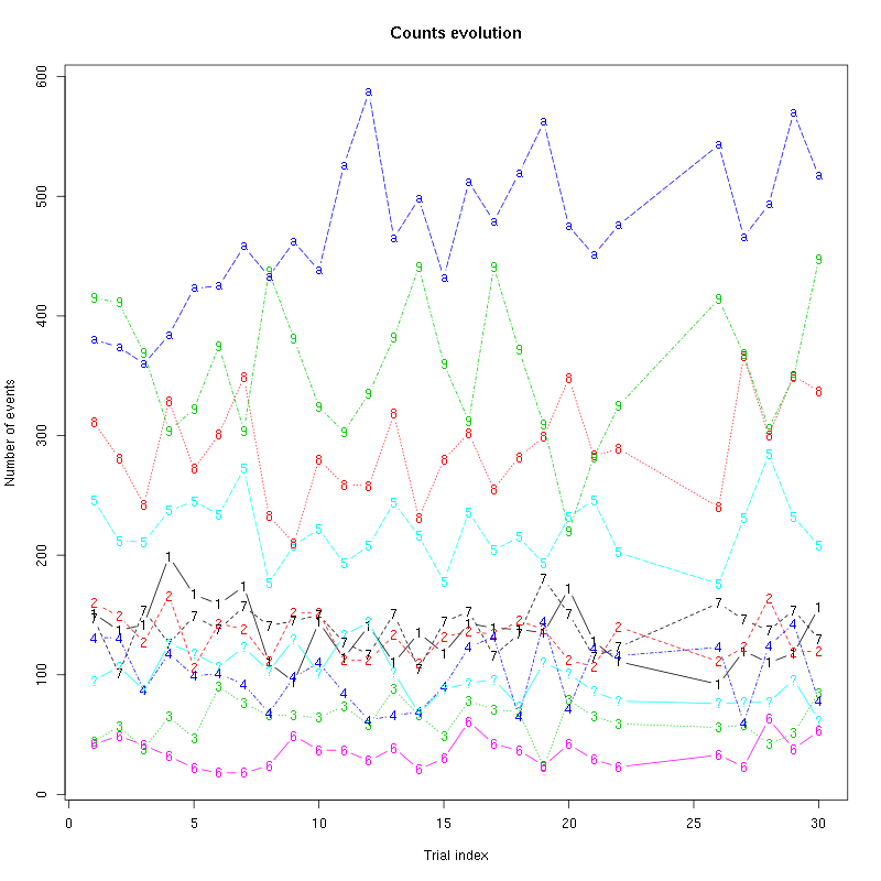
Figure 13: Evolution of the number of events attributed to each unit (1 to 9 and "a") or unclassified ("?") during the 30 trials of Spontaneous_2 for tetrode B.

The waveform evolution is:

waveform_evolution(a_Spontaneous_2_tetB,threshold_factor,matrix(1:10,nr=5))

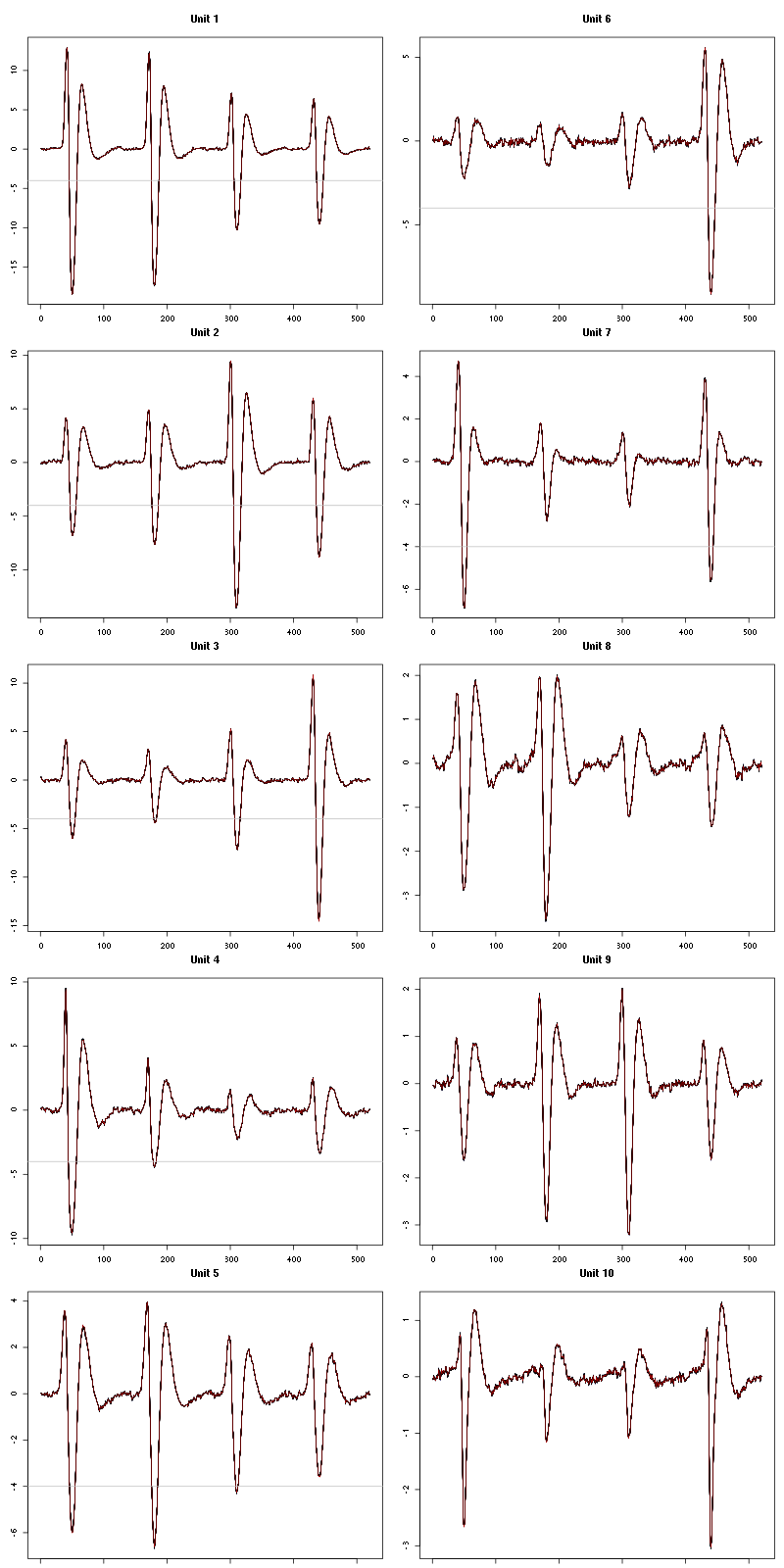
Figure 14: Evolution of the templates of each unit during the 30 trials with Spontaneous_2 for tetrode B.

The observed counting processes and inter spike intervals densities are:

cp_isi(a_Spontaneous_2_tetB,nbins=100)

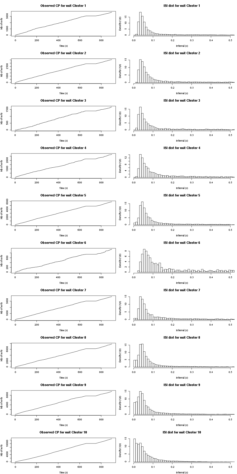
Figure 15: Observed counting processes, empirical inter spike interval distributions and raster plots for Spontaneous_1.

The BRT and RFT tests give for the first 6 units:

layout_matrix = matrix(0,nr=nbc-3,nc=nbc-3)
counter = 1
for (i in 1:(nbc-3))
    for (j in 1:(nbc-3))
        if (i != j) {
            layout_matrix[i,j] = counter
            counter = counter +1
        }
layout(layout_matrix)
par(mar=c(4,3,4,1))
for (i in 1:(nbc-3))
    for (j in 1:(nbc-3))
        if (i != j)
            test_rt(a_Spontaneous_2_tetB$spike_trains[[i]],
                    a_Spontaneous_2_tetB$spike_trains[[j]],
		    nbins=200, single_trial_duration=30,
                    ylab="",main=paste("Units",i,"and",j))

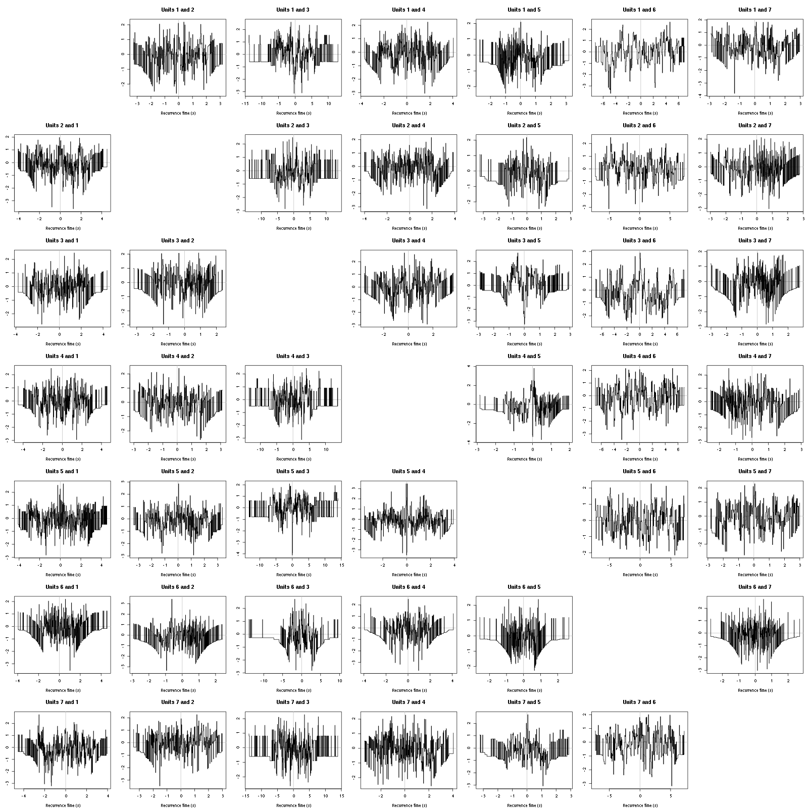
Figure 16: Graphical tests for the first 7 units of the Backward and Forward Reccurrence Times distribution against the null hypothesis (no interaction) during Spontaneous_2. If the null is correct, the curves should be IID draws from a standard normal distribution.

Still no clear signs of interactions.

4.3 Save results

Before analyzing the next set of trials we save the output of sort_many_trials to disk with:

save(a_Spontaneous_2_tetB,
     file=paste0("tetB_analysis/tetB_","Spontaneous_2","_summary_obj.rda"))

We write to disk the spike trains in text mode:

for (c_idx in 1:length(a_Spontaneous_2_tetB$spike_trains))
    cat(a_Spontaneous_2_tetB$spike_trains[[c_idx]],
        file=paste0("locust20010214_spike_trains/locust20010214_Spontaneous_2_tetB_u",c_idx,".txt"),sep="\n")

5 30 trials of `Spontaenous_1` backwards

We will carry out an analysis of the 30 trials of Spontaneous_2 backwards. The LabBook mentions that that noise is present at trials 11 and 21 so we skip these trials.

5.1 Do the job

a_Spontaneous_1_tetB=sort_many_trials(inter_trial_time=30*15000,
                                      get_data_fct=get_tetrode_data,
                                      stim_name="Spontaneous_1",
                                      trial_nbs=rev(c(1:10,12:20,22:30)),
                                      centers=a_Spontaneous_2_tetB$centers,
                                      counts=a_Spontaneous_2_tetB$counts,
                                      all_at_once_call_list=list(thres=threshold_factor*c(1,1,1,1), 
                                                                 filter_length_1=filter_length, filter_length=filter_length, 
                                                                 minimalDist_1=15, minimalDist=15, 
                                                                 before=c_before, after=c_after, 
                                                                 detection_cycle=c(0,0), verbose=1),
                                      layout_matrix=matrix(c(1,1:11),nr=6),new_weight_in_update=0.01
                                      )

***************
Doing now trial 30 of Spontaneous_1
The five number summary is:
       V1             V2             V3             V4      
 Min.   : 394   Min.   : 741   Min.   :1073   Min.   : 737  
 1st Qu.:2013   1st Qu.:2015   1st Qu.:2017   1st Qu.:2015  
 Median :2058   Median :2057   Median :2057   Median :2058  
 Mean   :2055   Mean   :2055   Mean   :2054   Mean   :2056  
 3rd Qu.:2102   3rd Qu.:2098   3rd Qu.:2095   3rd Qu.:2101  
 Max.   :3212   Max.   :2986   Max.   :2984   Max.   :3085  

Global counts at classification's end:
     Total  Cluster 1  Cluster 2  Cluster 3  Cluster 4  Cluster 5  Cluster 6 
      1930        145        147         62         68        186         23 
 Cluster 7  Cluster 8  Cluster 9 Cluster 10          ? 
       113        244        411        401        130 
Trial 30 done!
******************
***************
Doing now trial 29 of Spontaneous_1
The five number summary is:
       V1             V2             V3             V4      
 Min.   : 343   Min.   : 530   Min.   : 749   Min.   : 821  
 1st Qu.:2013   1st Qu.:2016   1st Qu.:2017   1st Qu.:2015  
 Median :2058   Median :2057   Median :2057   Median :2058  
 Mean   :2056   Mean   :2055   Mean   :2054   Mean   :2056  
 3rd Qu.:2102   3rd Qu.:2098   3rd Qu.:2095   3rd Qu.:2101  
 Max.   :3292   Max.   :3109   Max.   :2958   Max.   :3077  

Global counts at classification's end:
     Total  Cluster 1  Cluster 2  Cluster 3  Cluster 4  Cluster 5  Cluster 6 
      1790        100        182         61         69        192         32 
 Cluster 7  Cluster 8  Cluster 9 Cluster 10          ? 
       130        214        342        368        100 
Trial 29 done!
******************
***************
Doing now trial 28 of Spontaneous_1
The five number summary is:
       V1             V2             V3             V4      
 Min.   : 382   Min.   : 739   Min.   :1006   Min.   : 359  
 1st Qu.:2013   1st Qu.:2016   1st Qu.:2018   1st Qu.:2015  
 Median :2058   Median :2057   Median :2057   Median :2058  
 Mean   :2056   Mean   :2055   Mean   :2055   Mean   :2056  
 3rd Qu.:2102   3rd Qu.:2097   3rd Qu.:2094   3rd Qu.:2101  
 Max.   :3197   Max.   :3089   Max.   :2865   Max.   :3317  

Global counts at classification's end:
     Total  Cluster 1  Cluster 2  Cluster 3  Cluster 4  Cluster 5  Cluster 6 
      1819        118        153         52         78        205         31 
 Cluster 7  Cluster 8  Cluster 9 Cluster 10          ? 
       186        239        303        353        101 
Trial 28 done!
******************
***************
Doing now trial 27 of Spontaneous_1
The five number summary is:
       V1             V2             V3             V4      
 Min.   : 412   Min.   : 671   Min.   : 888   Min.   : 483  
 1st Qu.:2013   1st Qu.:2016   1st Qu.:2018   1st Qu.:2016  
 Median :2058   Median :2057   Median :2056   Median :2058  
 Mean   :2056   Mean   :2055   Mean   :2055   Mean   :2056  
 3rd Qu.:2102   3rd Qu.:2097   3rd Qu.:2094   3rd Qu.:2100  
 Max.   :3267   Max.   :3011   Max.   :2821   Max.   :3266  

Global counts at classification's end:
     Total  Cluster 1  Cluster 2  Cluster 3  Cluster 4  Cluster 5  Cluster 6 
      1718        126        115         58         56        200         46 
 Cluster 7  Cluster 8  Cluster 9 Cluster 10          ? 
       136        238        312        331        100 
Trial 27 done!
******************
***************
Doing now trial 26 of Spontaneous_1
The five number summary is:
       V1             V2             V3             V4      
 Min.   : 369   Min.   : 566   Min.   : 900   Min.   : 855  
 1st Qu.:2012   1st Qu.:2015   1st Qu.:2017   1st Qu.:2015  
 Median :2058   Median :2057   Median :2056   Median :2059  
 Mean   :2055   Mean   :2055   Mean   :2054   Mean   :2056  
 3rd Qu.:2103   3rd Qu.:2098   3rd Qu.:2094   3rd Qu.:2101  
 Max.   :3242   Max.   :3101   Max.   :2916   Max.   :3095  

Global counts at classification's end:
     Total  Cluster 1  Cluster 2  Cluster 3  Cluster 4  Cluster 5  Cluster 6 
      1923        128        128         61        118        227         55 
 Cluster 7  Cluster 8  Cluster 9 Cluster 10          ? 
       152        260        359        318        117 
Trial 26 done!
******************
***************
Doing now trial 25 of Spontaneous_1
The five number summary is:
       V1             V2             V3             V4      
 Min.   : 587   Min.   : 877   Min.   :1091   Min.   : 743  
 1st Qu.:2013   1st Qu.:2016   1st Qu.:2017   1st Qu.:2015  
 Median :2058   Median :2057   Median :2056   Median :2058  
 Mean   :2055   Mean   :2055   Mean   :2054   Mean   :2056  
 3rd Qu.:2103   3rd Qu.:2097   3rd Qu.:2094   3rd Qu.:2101  
 Max.   :3188   Max.   :2939   Max.   :2733   Max.   :3093  

Global counts at classification's end:
     Total  Cluster 1  Cluster 2  Cluster 3  Cluster 4  Cluster 5  Cluster 6 
      1767        127        138         57         80        221         27 
 Cluster 7  Cluster 8  Cluster 9 Cluster 10          ? 
       159        243        310        313         92 
Trial 25 done!
******************
***************
Doing now trial 24 of Spontaneous_1
The five number summary is:
       V1             V2             V3             V4      
 Min.   : 492   Min.   : 702   Min.   :1130   Min.   : 596  
 1st Qu.:2013   1st Qu.:2017   1st Qu.:2018   1st Qu.:2016  
 Median :2058   Median :2057   Median :2057   Median :2058  
 Mean   :2056   Mean   :2055   Mean   :2055   Mean   :2056  
 3rd Qu.:2102   3rd Qu.:2097   3rd Qu.:2094   3rd Qu.:2100  
 Max.   :3233   Max.   :3007   Max.   :2723   Max.   :3095  

Global counts at classification's end:
     Total  Cluster 1  Cluster 2  Cluster 3  Cluster 4  Cluster 5  Cluster 6 
      1738         91        110         75         68        182         29 
 Cluster 7  Cluster 8  Cluster 9 Cluster 10          ? 
       171        261        333        337         81 
Trial 24 done!
******************
***************
Doing now trial 23 of Spontaneous_1
The five number summary is:
       V1             V2             V3             V4      
 Min.   : 362   Min.   : 736   Min.   :1065   Min.   : 430  
 1st Qu.:2013   1st Qu.:2016   1st Qu.:2018   1st Qu.:2015  
 Median :2058   Median :2057   Median :2057   Median :2058  
 Mean   :2056   Mean   :2055   Mean   :2055   Mean   :2056  
 3rd Qu.:2102   3rd Qu.:2097   3rd Qu.:2094   3rd Qu.:2100  
 Max.   :3241   Max.   :3003   Max.   :2790   Max.   :3203  

Global counts at classification's end:
     Total  Cluster 1  Cluster 2  Cluster 3  Cluster 4  Cluster 5  Cluster 6 
      1746        103        114         85         75        172         28 
 Cluster 7  Cluster 8  Cluster 9 Cluster 10          ? 
       151        223        409        314         72 
Trial 23 done!
******************
***************
Doing now trial 22 of Spontaneous_1
The five number summary is:
       V1             V2             V3             V4      
 Min.   : 517   Min.   : 779   Min.   :1170   Min.   : 759  
 1st Qu.:2013   1st Qu.:2016   1st Qu.:2017   1st Qu.:2015  
 Median :2058   Median :2057   Median :2056   Median :2058  
 Mean   :2055   Mean   :2055   Mean   :2054   Mean   :2056  
 3rd Qu.:2102   3rd Qu.:2098   3rd Qu.:2094   3rd Qu.:2100  
 Max.   :3290   Max.   :3095   Max.   :2769   Max.   :3131  

Global counts at classification's end:
     Total  Cluster 1  Cluster 2  Cluster 3  Cluster 4  Cluster 5  Cluster 6 
      1744        139        104         34        100        238         29 
 Cluster 7  Cluster 8  Cluster 9 Cluster 10          ? 
       122        276        346        283         73 
Trial 22 done!
******************
***************
Doing now trial 20 of Spontaneous_1
The five number summary is:
       V1             V2             V3             V4      
 Min.   : 552   Min.   : 792   Min.   : 970   Min.   : 830  
 1st Qu.:2013   1st Qu.:2016   1st Qu.:2017   1st Qu.:2016  
 Median :2058   Median :2057   Median :2057   Median :2058  
 Mean   :2056   Mean   :2055   Mean   :2054   Mean   :2056  
 3rd Qu.:2102   3rd Qu.:2098   3rd Qu.:2094   3rd Qu.:2100  
 Max.   :3186   Max.   :2980   Max.   :2858   Max.   :3093  

Global counts at classification's end:
     Total  Cluster 1  Cluster 2  Cluster 3  Cluster 4  Cluster 5  Cluster 6 
      1851        133        138         73         47        175         44 
 Cluster 7  Cluster 8  Cluster 9 Cluster 10          ? 
       117        329        390        269        136 
Trial 20 done!
******************
***************
Doing now trial 19 of Spontaneous_1
The five number summary is:
       V1             V2             V3             V4      
 Min.   : 473   Min.   : 656   Min.   : 869   Min.   : 864  
 1st Qu.:2013   1st Qu.:2015   1st Qu.:2017   1st Qu.:2015  
 Median :2058   Median :2057   Median :2056   Median :2058  
 Mean   :2056   Mean   :2055   Mean   :2054   Mean   :2056  
 3rd Qu.:2102   3rd Qu.:2098   3rd Qu.:2095   3rd Qu.:2101  
 Max.   :3273   Max.   :3158   Max.   :2926   Max.   :3241  

Global counts at classification's end:
     Total  Cluster 1  Cluster 2  Cluster 3  Cluster 4  Cluster 5  Cluster 6 
      1859        149        140         17        104        275         30 
 Cluster 7  Cluster 8  Cluster 9 Cluster 10          ? 
       120        243        332        284        165 
Trial 19 done!
******************
***************
Doing now trial 18 of Spontaneous_1
The five number summary is:
       V1             V2             V3             V4      
 Min.   : 518   Min.   : 781   Min.   :1089   Min.   : 377  
 1st Qu.:2013   1st Qu.:2015   1st Qu.:2017   1st Qu.:2015  
 Median :2058   Median :2057   Median :2057   Median :2058  
 Mean   :2056   Mean   :2055   Mean   :2054   Mean   :2056  
 3rd Qu.:2102   3rd Qu.:2098   3rd Qu.:2095   3rd Qu.:2101  
 Max.   :3261   Max.   :3000   Max.   :2751   Max.   :3275  

Global counts at classification's end:
     Total  Cluster 1  Cluster 2  Cluster 3  Cluster 4  Cluster 5  Cluster 6 
      1835        129        148         38         58        246         57 
 Cluster 7  Cluster 8  Cluster 9 Cluster 10          ? 
       194        255        330        239        141 
Trial 18 done!
******************
***************
Doing now trial 17 of Spontaneous_1
The five number summary is:
       V1             V2             V3             V4      
 Min.   : 691   Min.   : 813   Min.   :1043   Min.   : 865  
 1st Qu.:2014   1st Qu.:2016   1st Qu.:2017   1st Qu.:2015  
 Median :2058   Median :2057   Median :2056   Median :2058  
 Mean   :2056   Mean   :2055   Mean   :2055   Mean   :2056  
 3rd Qu.:2101   3rd Qu.:2097   3rd Qu.:2094   3rd Qu.:2100  
 Max.   :3154   Max.   :2910   Max.   :2679   Max.   :3093  

Global counts at classification's end:
     Total  Cluster 1  Cluster 2  Cluster 3  Cluster 4  Cluster 5  Cluster 6 
      1728        129        133         30         48        210         41 
 Cluster 7  Cluster 8  Cluster 9 Cluster 10          ? 
       140        263        356        268        110 
Trial 17 done!
******************
***************
Doing now trial 16 of Spontaneous_1
The five number summary is:
       V1             V2             V3             V4      
 Min.   : 545   Min.   : 990   Min.   :1203   Min.   : 663  
 1st Qu.:2014   1st Qu.:2016   1st Qu.:2017   1st Qu.:2016  
 Median :2058   Median :2057   Median :2056   Median :2058  
 Mean   :2056   Mean   :2055   Mean   :2054   Mean   :2056  
 3rd Qu.:2101   3rd Qu.:2097   3rd Qu.:2094   3rd Qu.:2100  
 Max.   :3104   Max.   :2898   Max.   :2648   Max.   :3121  

Global counts at classification's end:
     Total  Cluster 1  Cluster 2  Cluster 3  Cluster 4  Cluster 5  Cluster 6 
      1688        113        139         33         59        207         42 
 Cluster 7  Cluster 8  Cluster 9 Cluster 10          ? 
       163        206        366        246        114 
Trial 16 done!
******************
***************
Doing now trial 15 of Spontaneous_1
The five number summary is:
       V1             V2             V3             V4      
 Min.   : 644   Min.   : 986   Min.   :1138   Min.   : 754  
 1st Qu.:2013   1st Qu.:2016   1st Qu.:2017   1st Qu.:2015  
 Median :2058   Median :2057   Median :2056   Median :2058  
 Mean   :2055   Mean   :2055   Mean   :2054   Mean   :2056  
 3rd Qu.:2101   3rd Qu.:2097   3rd Qu.:2094   3rd Qu.:2100  
 Max.   :3180   Max.   :3002   Max.   :2687   Max.   :3088  

Global counts at classification's end:
     Total  Cluster 1  Cluster 2  Cluster 3  Cluster 4  Cluster 5  Cluster 6 
      1724        119        130         39         55        200         25 
 Cluster 7  Cluster 8  Cluster 9 Cluster 10          ? 
       141        237        387        275        116 
Trial 15 done!
******************
***************
Doing now trial 14 of Spontaneous_1
The five number summary is:
       V1             V2             V3             V4      
 Min.   : 541   Min.   : 778   Min.   : 975   Min.   : 882  
 1st Qu.:2014   1st Qu.:2016   1st Qu.:2018   1st Qu.:2015  
 Median :2058   Median :2057   Median :2057   Median :2058  
 Mean   :2056   Mean   :2055   Mean   :2054   Mean   :2056  
 3rd Qu.:2101   3rd Qu.:2097   3rd Qu.:2094   3rd Qu.:2100  
 Max.   :3174   Max.   :3040   Max.   :2734   Max.   :3133  

Global counts at classification's end:
     Total  Cluster 1  Cluster 2  Cluster 3  Cluster 4  Cluster 5  Cluster 6 
      1730        110        130         53         51        180         30 
 Cluster 7  Cluster 8  Cluster 9 Cluster 10          ? 
       140        264        398        269        105 
Trial 14 done!
******************
***************
Doing now trial 13 of Spontaneous_1
The five number summary is:
       V1             V2             V3             V4      
 Min.   : 531   Min.   : 815   Min.   :1188   Min.   : 797  
 1st Qu.:2013   1st Qu.:2017   1st Qu.:2018   1st Qu.:2016  
 Median :2058   Median :2057   Median :2056   Median :2058  
 Mean   :2056   Mean   :2055   Mean   :2054   Mean   :2056  
 3rd Qu.:2101   3rd Qu.:2097   3rd Qu.:2094   3rd Qu.:2100  
 Max.   :3179   Max.   :2946   Max.   :2670   Max.   :3213  

Global counts at classification's end:
     Total  Cluster 1  Cluster 2  Cluster 3  Cluster 4  Cluster 5  Cluster 6 
      1760        104        124         33         85        202         35 
 Cluster 7  Cluster 8  Cluster 9 Cluster 10          ? 
       192        222        383        264        116 
Trial 13 done!
******************
***************
Doing now trial 12 of Spontaneous_1
The five number summary is:
       V1             V2             V3             V4      
 Min.   : 490   Min.   : 771   Min.   : 975   Min.   : 647  
 1st Qu.:2013   1st Qu.:2016   1st Qu.:2018   1st Qu.:2015  
 Median :2058   Median :2057   Median :2056   Median :2058  
 Mean   :2056   Mean   :2055   Mean   :2054   Mean   :2056  
 3rd Qu.:2102   3rd Qu.:2097   3rd Qu.:2094   3rd Qu.:2101  
 Max.   :3396   Max.   :3005   Max.   :2709   Max.   :3251  

Global counts at classification's end:
     Total  Cluster 1  Cluster 2  Cluster 3  Cluster 4  Cluster 5  Cluster 6 
      1867        161        122         45        119        203         27 
 Cluster 7  Cluster 8  Cluster 9 Cluster 10          ? 
       154        270        325        322        119 
Trial 12 done!
******************
***************
Doing now trial 10 of Spontaneous_1
The five number summary is:
       V1             V2             V3             V4      
 Min.   : 721   Min.   : 993   Min.   :1250   Min.   : 808  
 1st Qu.:2014   1st Qu.:2017   1st Qu.:2018   1st Qu.:2016  
 Median :2058   Median :2057   Median :2056   Median :2058  
 Mean   :2056   Mean   :2055   Mean   :2055   Mean   :2056  
 3rd Qu.:2100   3rd Qu.:2096   3rd Qu.:2093   3rd Qu.:2099  
 Max.   :3103   Max.   :2868   Max.   :2631   Max.   :3095  

Global counts at classification's end:
     Total  Cluster 1  Cluster 2  Cluster 3  Cluster 4  Cluster 5  Cluster 6 
      1765         88        124         35         34        125         29 
 Cluster 7  Cluster 8  Cluster 9 Cluster 10          ? 
       134        333        341        327        195 
Trial 10 done!
******************
***************
Doing now trial 9 of Spontaneous_1
The five number summary is:
       V1             V2             V3             V4      
 Min.   : 637   Min.   : 921   Min.   : 976   Min.   : 315  
 1st Qu.:2014   1st Qu.:2016   1st Qu.:2018   1st Qu.:2016  
 Median :2058   Median :2057   Median :2056   Median :2058  
 Mean   :2056   Mean   :2055   Mean   :2055   Mean   :2056  
 3rd Qu.:2101   3rd Qu.:2097   3rd Qu.:2094   3rd Qu.:2100  
 Max.   :4071   Max.   :4071   Max.   :4074   Max.   :4074  

Global counts at classification's end:
     Total  Cluster 1  Cluster 2  Cluster 3  Cluster 4  Cluster 5  Cluster 6 
      1926        154        129         60         50        153         34 
 Cluster 7  Cluster 8  Cluster 9 Cluster 10          ? 
       133        309        303        361        240 
Trial 9 done!
******************
***************
Doing now trial 8 of Spontaneous_1
The five number summary is:
       V1             V2             V3             V4      
 Min.   : 552   Min.   : 789   Min.   : 977   Min.   : 690  
 1st Qu.:2014   1st Qu.:2017   1st Qu.:2018   1st Qu.:2016  
 Median :2058   Median :2057   Median :2056   Median :2058  
 Mean   :2056   Mean   :2055   Mean   :2055   Mean   :2056  
 3rd Qu.:2101   3rd Qu.:2096   3rd Qu.:2094   3rd Qu.:2099  
 Max.   :3106   Max.   :2880   Max.   :2813   Max.   :3236  

Global counts at classification's end:
     Total  Cluster 1  Cluster 2  Cluster 3  Cluster 4  Cluster 5  Cluster 6 
      1720        113        104         40         68        140         22 
 Cluster 7  Cluster 8  Cluster 9 Cluster 10          ? 
       155        257        319        336        166 
Trial 8 done!
******************
***************
Doing now trial 7 of Spontaneous_1
The five number summary is:
       V1             V2             V3             V4      
 Min.   : 492   Min.   : 957   Min.   :1112   Min.   : 587  
 1st Qu.:2014   1st Qu.:2016   1st Qu.:2018   1st Qu.:2015  
 Median :2058   Median :2057   Median :2056   Median :2058  
 Mean   :2056   Mean   :2055   Mean   :2055   Mean   :2056  
 3rd Qu.:2101   3rd Qu.:2097   3rd Qu.:2094   3rd Qu.:2100  
 Max.   :3367   Max.   :3004   Max.   :2744   Max.   :3156  

Global counts at classification's end:
     Total  Cluster 1  Cluster 2  Cluster 3  Cluster 4  Cluster 5  Cluster 6 
      1835        116        145         47         47        158         31 
 Cluster 7  Cluster 8  Cluster 9 Cluster 10          ? 
       149        298        316        345        183 
Trial 7 done!
******************
***************
Doing now trial 6 of Spontaneous_1
The five number summary is:
       V1             V2             V3             V4      
 Min.   : 672   Min.   :1002   Min.   :1264   Min.   : 763  
 1st Qu.:2014   1st Qu.:2016   1st Qu.:2018   1st Qu.:2016  
 Median :2058   Median :2057   Median :2056   Median :2058  
 Mean   :2056   Mean   :2055   Mean   :2055   Mean   :2056  
 3rd Qu.:2101   3rd Qu.:2096   3rd Qu.:2094   3rd Qu.:2099  
 Max.   :3060   Max.   :2879   Max.   :2704   Max.   :3255  

Global counts at classification's end:
     Total  Cluster 1  Cluster 2  Cluster 3  Cluster 4  Cluster 5  Cluster 6 
      1810        106        100         52         65        116         37 
 Cluster 7  Cluster 8  Cluster 9 Cluster 10          ? 
       129        282        328        412        183 
Trial 6 done!
******************
***************
Doing now trial 5 of Spontaneous_1
The five number summary is:
       V1             V2             V3             V4      
 Min.   : 600   Min.   : 801   Min.   :1080   Min.   : 738  
 1st Qu.:2015   1st Qu.:2017   1st Qu.:2018   1st Qu.:2016  
 Median :2058   Median :2057   Median :2056   Median :2058  
 Mean   :2056   Mean   :2055   Mean   :2055   Mean   :2056  
 3rd Qu.:2100   3rd Qu.:2096   3rd Qu.:2093   3rd Qu.:2099  
 Max.   :3162   Max.   :2985   Max.   :2854   Max.   :3103  

Global counts at classification's end:
     Total  Cluster 1  Cluster 2  Cluster 3  Cluster 4  Cluster 5  Cluster 6 
      1701        107         88         43         64        100         34 
 Cluster 7  Cluster 8  Cluster 9 Cluster 10          ? 
       142        327        323        308        165 
Trial 5 done!
******************
***************
Doing now trial 4 of Spontaneous_1
The five number summary is:
       V1             V2             V3             V4      
 Min.   : 712   Min.   : 971   Min.   :1088   Min.   : 763  
 1st Qu.:2014   1st Qu.:2017   1st Qu.:2018   1st Qu.:2016  
 Median :2058   Median :2057   Median :2056   Median :2058  
 Mean   :2056   Mean   :2055   Mean   :2054   Mean   :2056  
 3rd Qu.:2101   3rd Qu.:2096   3rd Qu.:2094   3rd Qu.:2100  
 Max.   :3196   Max.   :2883   Max.   :2740   Max.   :3245  

Global counts at classification's end:
     Total  Cluster 1  Cluster 2  Cluster 3  Cluster 4  Cluster 5  Cluster 6 
      1795        128        137         66         65         99         20 
 Cluster 7  Cluster 8  Cluster 9 Cluster 10          ? 
       138        273        376        308        185 
Trial 4 done!
******************
***************
Doing now trial 3 of Spontaneous_1
The five number summary is:
       V1             V2             V3             V4      
 Min.   : 726   Min.   : 985   Min.   :1354   Min.   : 829  
 1st Qu.:2014   1st Qu.:2017   1st Qu.:2018   1st Qu.:2016  
 Median :2058   Median :2057   Median :2056   Median :2058  
 Mean   :2056   Mean   :2055   Mean   :2054   Mean   :2056  
 3rd Qu.:2101   3rd Qu.:2096   3rd Qu.:2094   3rd Qu.:2099  
 Max.   :3118   Max.   :2873   Max.   :2659   Max.   :3056  

Global counts at classification's end:
     Total  Cluster 1  Cluster 2  Cluster 3  Cluster 4  Cluster 5  Cluster 6 
      1801         99        152         38         67        101         24 
 Cluster 7  Cluster 8  Cluster 9 Cluster 10          ? 
       163        303        383        313        158 
Trial 3 done!
******************
***************
Doing now trial 2 of Spontaneous_1
The five number summary is:
       V1             V2             V3             V4      
 Min.   : 699   Min.   : 972   Min.   :1209   Min.   : 466  
 1st Qu.:2014   1st Qu.:2017   1st Qu.:2018   1st Qu.:2016  
 Median :2058   Median :2057   Median :2056   Median :2058  
 Mean   :2056   Mean   :2055   Mean   :2055   Mean   :2056  
 3rd Qu.:2100   3rd Qu.:2096   3rd Qu.:2094   3rd Qu.:2099  
 Max.   :3178   Max.   :2922   Max.   :2651   Max.   :3164  

Global counts at classification's end:
     Total  Cluster 1  Cluster 2  Cluster 3  Cluster 4  Cluster 5  Cluster 6 
      1718        102        103         48         54         88         44 
 Cluster 7  Cluster 8  Cluster 9 Cluster 10          ? 
       178        287        383        315        116 
Trial 2 done!
******************
***************
Doing now trial 1 of Spontaneous_1
The five number summary is:
       V1             V2             V3             V4      
 Min.   : 566   Min.   : 890   Min.   :1158   Min.   : 758  
 1st Qu.:2014   1st Qu.:2016   1st Qu.:2017   1st Qu.:2015  
 Median :2058   Median :2057   Median :2056   Median :2058  
 Mean   :2055   Mean   :2055   Mean   :2055   Mean   :2056  
 3rd Qu.:2101   3rd Qu.:2097   3rd Qu.:2094   3rd Qu.:2099  
 Max.   :3159   Max.   :2914   Max.   :2696   Max.   :3179  

Global counts at classification's end:
     Total  Cluster 1  Cluster 2  Cluster 3  Cluster 4  Cluster 5  Cluster 6 
      1807         94        125         32         66        139         31 
 Cluster 7  Cluster 8  Cluster 9 Cluster 10          ? 
       181        280        387        350        122 
Trial 1 done!
******************

5.2 Diagnostic plots

The counts evolution is:

counts_evolution(a_Spontaneous_1_tetB)

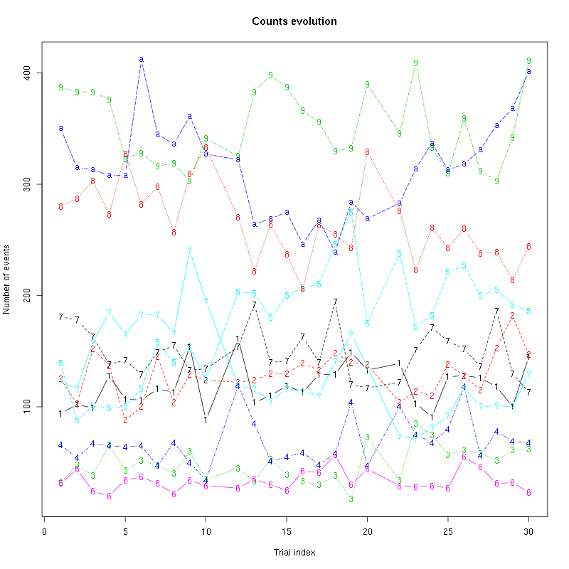
Figure 17: Evolution of the number of events attributed to each unit (1 to 9and "a") or unclassified ("?") during the 30 trials of Spontaneous_1 for tetrode B.

The waveform evolution is:

waveform_evolution(a_Spontaneous_1_tetB,threshold_factor,matrix(1:10,nr=5))

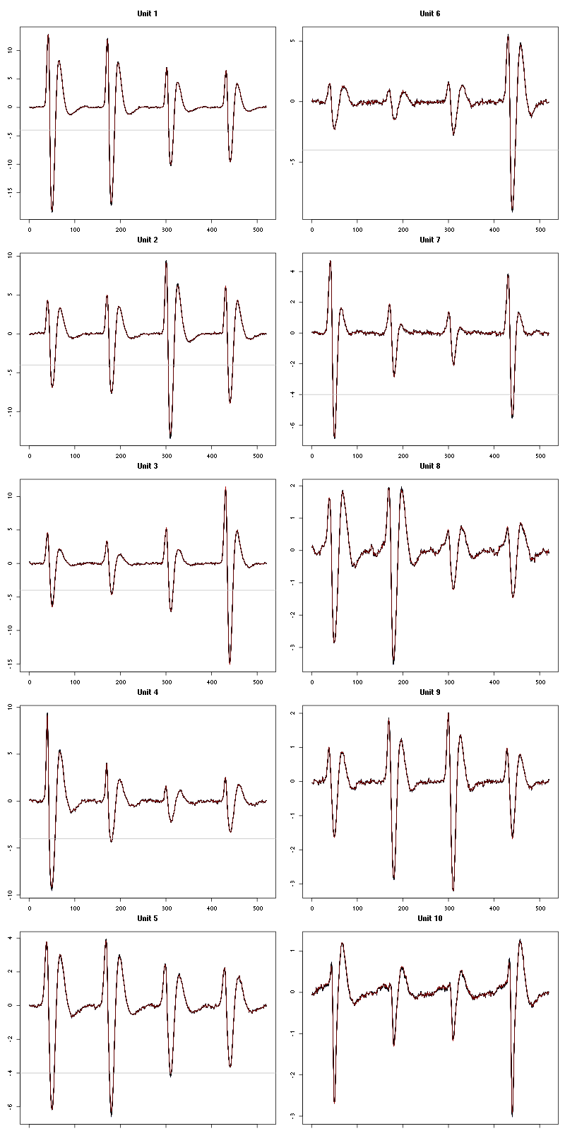
Figure 18: Evolution of the templates of each unit during the 30-2 trials of Spontaneous_1 for tetrode B.

The observed counting processes and inter spike intervals densities are:

cp_isi(a_Spontaneous_1_tetB,nbins=100)

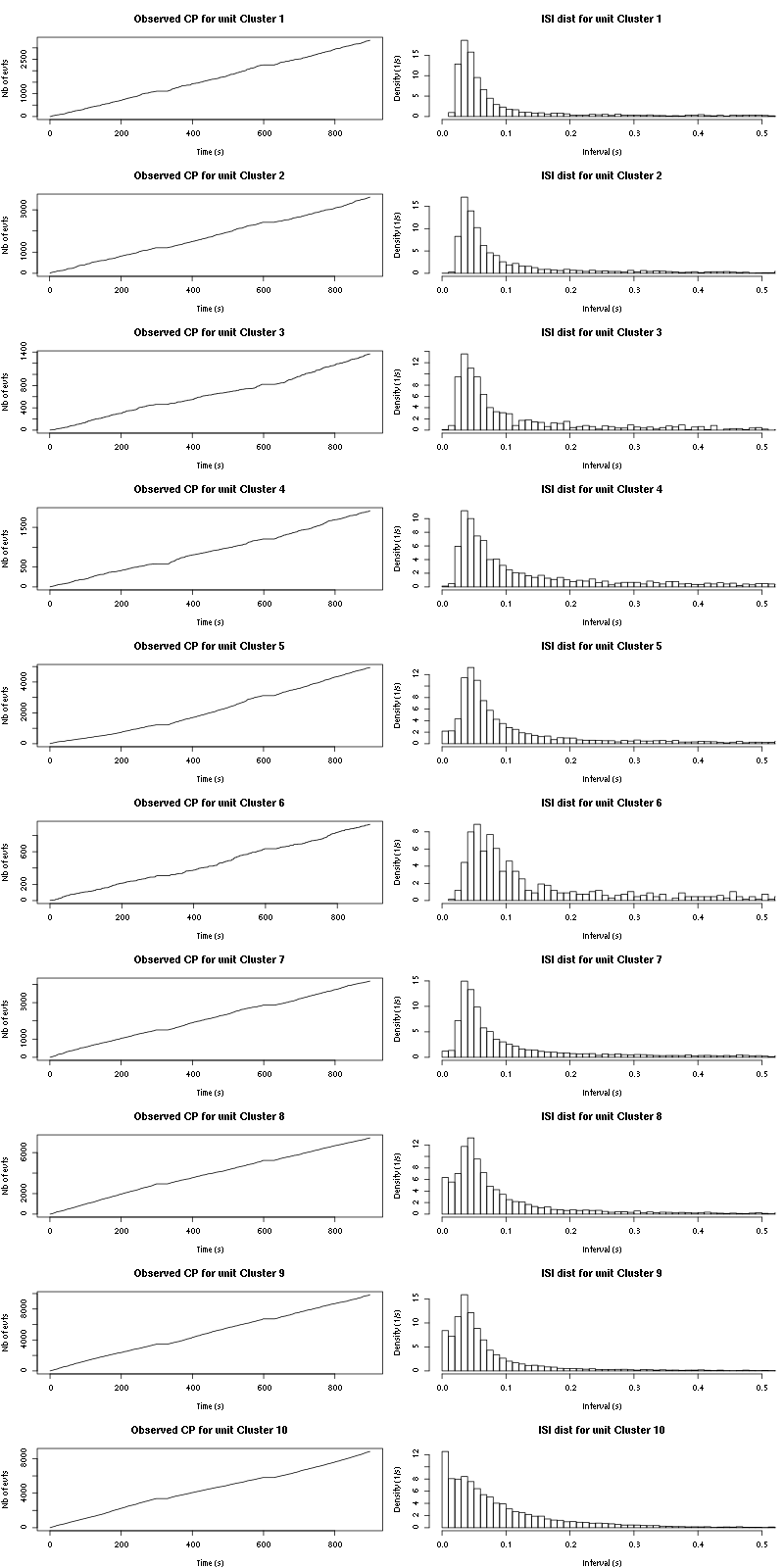
Figure 19: Observed counting processes and empirical inter spike interval distributions for Spontaneous_1.

The BRT and RFT tests give for the first 7 units:

layout_matrix = matrix(0,nr=nbc-3,nc=nbc-3)
counter = 1
for (i in 1:(nbc-3))
    for (j in 1:(nbc-3))
        if (i != j) {
            layout_matrix[i,j] = counter
            counter = counter +1
        }
layout(layout_matrix)
par(mar=c(4,3,4,1))
for (i in 1:(nbc-3))
    for (j in 1:(nbc-3))
        if (i != j)
            test_rt(a_Spontaneous_1_tetB$spike_trains[[i]],
                    a_Spontaneous_1_tetB$spike_trains[[j]],
		    nbins=200,single_trial_duration=30,
                    ylab="",main=paste("Units",i,"and",j))

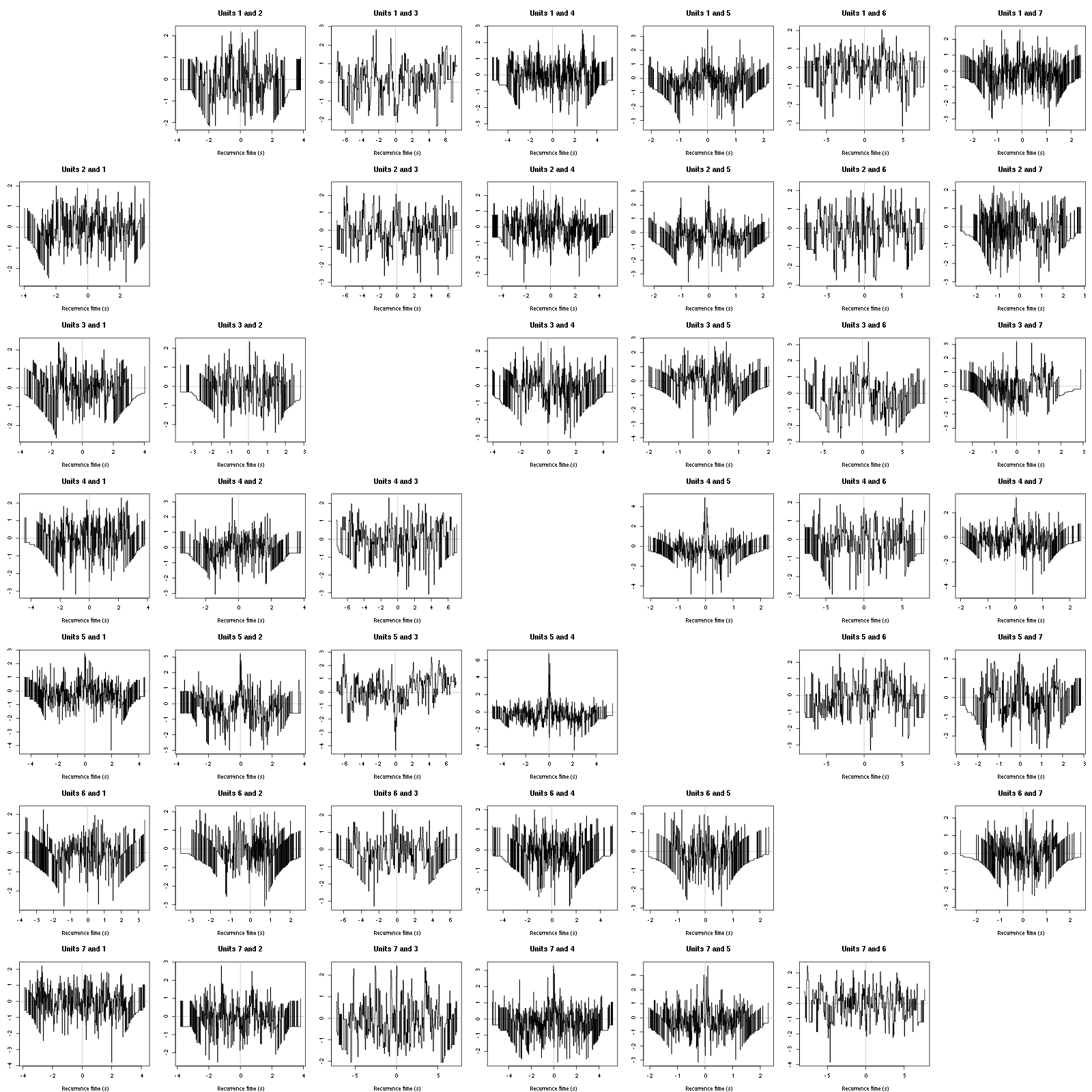
Figure 20: Graphical tests for the first 7 units of the Backward and Forward Reccurrence Times distribution against the null hypothesis (no interaction) during Spontaenous_1. If the null is correct, the curves should be IID draws from a standard normal distribution.

5.3 Save results

Before analyzing the next set of trials we save the output of sort_many_trials to disk with:

save(a_Spontaneous_1_tetB,
     file=paste0("tetB_analysis/tetB_","Spontaneous_1","_summary_obj.rda"))

We write to disk the spike trains in text mode:

for (c_idx in 1:length(a_Spontaneous_1_tetB$spike_trains))
    cat(a_Spontaneous_1_tetB$spike_trains[[c_idx]],
        file=paste0("locust20010214_spike_trains/locust20010214_Spontaneous_1_tetB_u",c_idx,".txt"),sep="\n")

6 25 trials with `Cis-3-Hexen-1-ol` (`C3H_1`)

We will carry out an analysis of the 25 trials from C3H_1.

6.1 Do the job

We do not print out the output to save space.

a_C3H_1_tetB=sort_many_trials(inter_trial_time=30*15000,
                              get_data_fct=get_tetrode_data,
                              stim_name="C3H_1",
                              trial_nbs=1:25,
                              centers=aao$centers,
                              counts=aao$counts,
                              all_at_once_call_list=list(thres=threshold_factor*c(1,1,1,1), 
                                                         filter_length_1=filter_length, filter_length=filter_length, 
                                                         minimalDist_1=15, minimalDist=15, 
                                                         before=c_before, after=c_after, 
                                                         detection_cycle=c(0,0), verbose=1),
                              layout_matrix=matrix(c(1,1:11),nr=6),new_weight_in_update=0.01
                              )

6.2 Diagnostic plots

The counts evolution is:

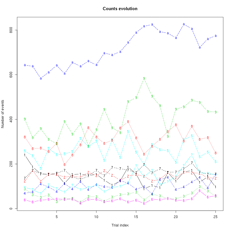
Figure 21: Evolution of the number of events attributed to each unit (1 to 9 and "a") or unclassified ("?") during the 30 trials of C3H_1 for tetrode B.

The waveform evolution is:

waveform_evolution(a_C3H_1_tetB,threshold_factor,matrix(1:10,nr=5))

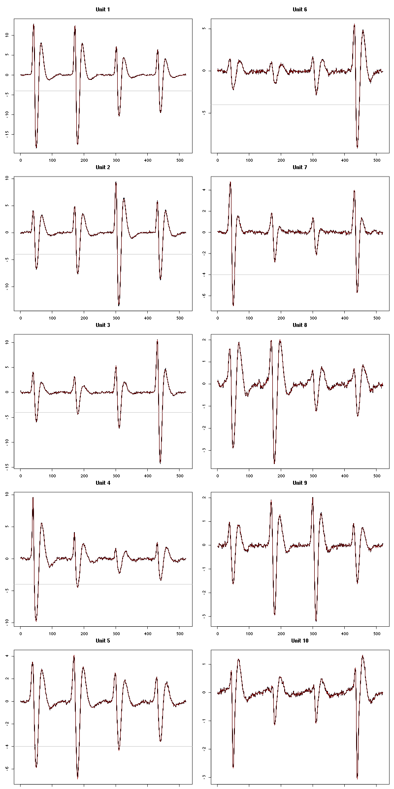
Figure 22: Evolution of the templates of each unit during the 25 trials of C3H_1 for stereode Ca.

The observed counting processes, inter spike intervals densities and raster plots are:

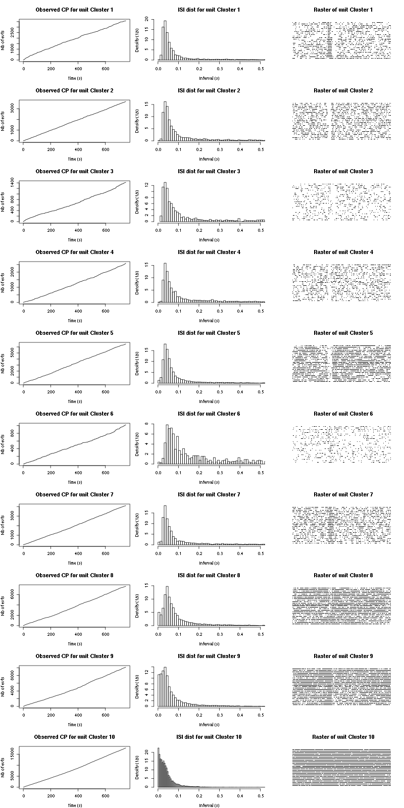
Figure 23: Observed counting processes, empirical inter spike interval distributions and raster plots for C3H_1.

The BRT and RFT tests give for the first 7 units:

layout_matrix = matrix(0,nr=nbc-3,nc=nbc-3)
counter = 1
for (i in 1:(nbc-3))
    for (j in 1:(nbc-3))
        if (i != j) {
            layout_matrix[i,j] = counter
            counter = counter +1
        }
layout(layout_matrix)
par(mar=c(4,3,4,1))
for (i in 1:(nbc-3))
    for (j in 1:(nbc-3))
        if (i != j)
            test_rt(a_C3H_1_tetB$spike_trains[[i]],
                    a_C3H_1_tetB$spike_trains[[j]],
		    nbins=200,single_trial_duration=30,
                    ylab="",main=paste("Units",i,"and",j))

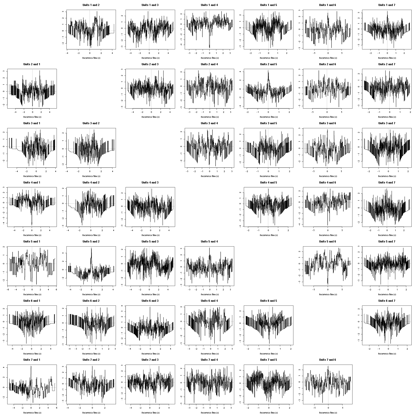
Figure 24: Graphical tests for the first 7 units of the Backward and Forward Reccurrence Times distribution against the null hypothesis (no interaction) during Spontaenous_1. If the null is correct, the curves should be IID draws from a standard normal distribution.

6.3 Save results

Before analyzing the next set of trials we save the output of sort_many_trials to disk with:

save(a_C3H_1_tetB,
     file=paste0("tetB_analysis/tetB_","C3H_1","_summary_obj.rda"))

We write to disk the spike trains in text mode:

for (c_idx in 1:length(a_C3H_1_tetB$spike_trains))
    if (!is.null(a_C3H_1_tetB$spike_trains[[c_idx]]))
        cat(a_C3H_1_tetB$spike_trains[[c_idx]],
	    file=paste0("locust20010214_spike_trains/locust20010214_C3H_1_tetB_u",c_idx,".txt"),sep="\n")

7 25 trials with `Citral`

We will carry out an analysis of the 25 trials from Citral_1.

7.1 Do the job

stim_name = "Citral_1"
a_Citral_1_tetB=sort_many_trials(inter_trial_time=30*15000,
                                 get_data_fct=get_tetrode_data,
                                 stim_name=stim_name,
                                 trial_nbs=1:25,
                                 centers=a_C3H_1_tetB$centers,
                                 counts=a_C3H_1_tetB$counts,
                                 all_at_once_call_list=list(thres=threshold_factor*c(1,1,1,1), 
                                                            filter_length_1=filter_length, filter_length=filter_length, 
                                                            minimalDist_1=15, minimalDist=15, 
                                                            before=c_before, after=c_after, 
                                                            detection_cycle=c(0,0), verbose=1),
                                 layout_matrix=matrix(c(1,1:11),nr=6),new_weight_in_update=0.01
                                 )

7.2 Diagnostic plots

The counts evolution is:

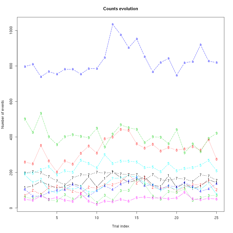
Figure 25: Evolution of the number of events attributed to each unit (1 to 9 and "a") or unclassified ("?") during the 25 trials of Citral_1 for tetrodeB.

The waveform evolution is:

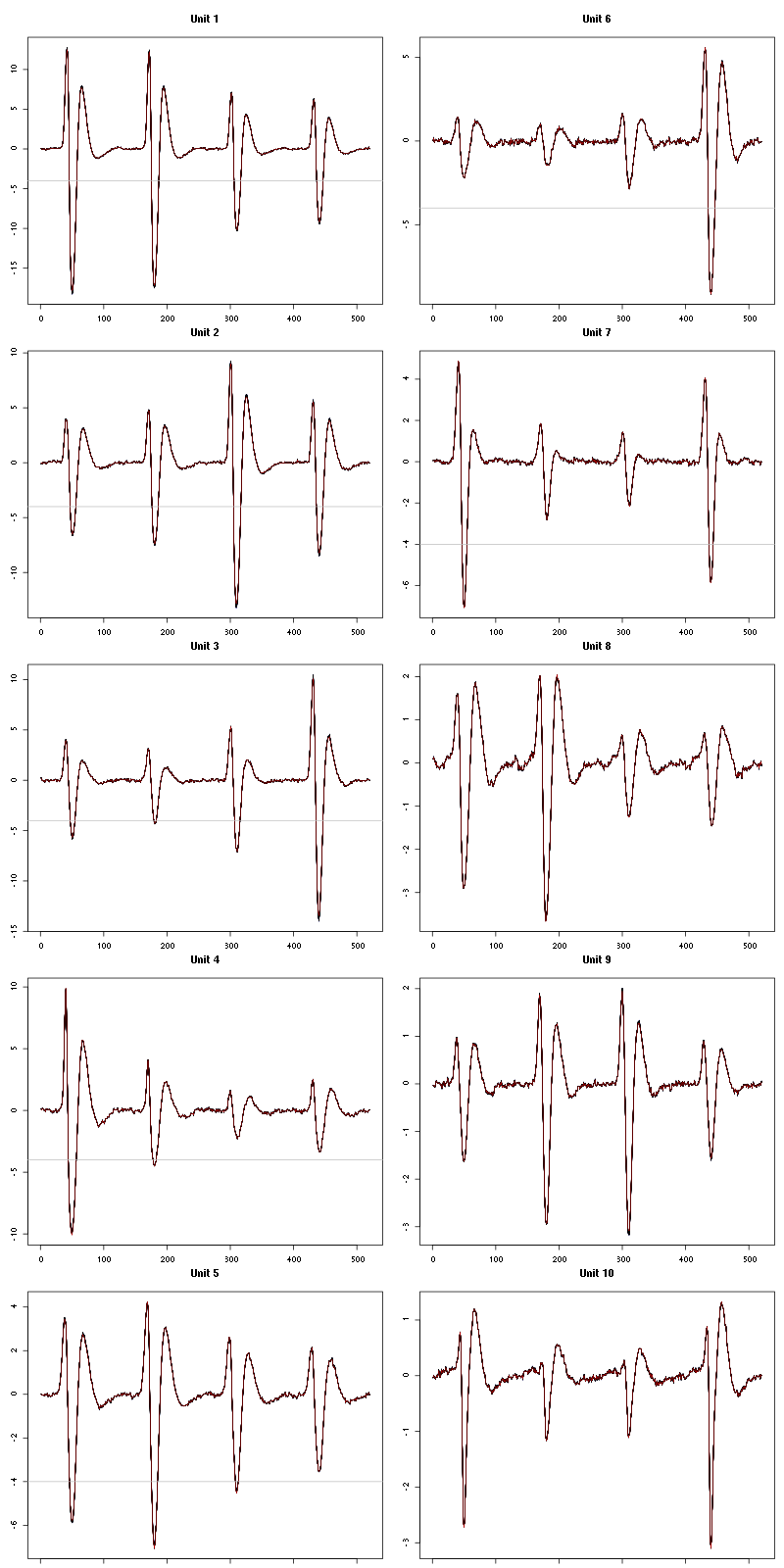
Figure 26: Evolution of the templates of each unit during the 25 trials of Citral for tetrodeB.

The observed counting processes, inter spike intervals densities and raster plots are:

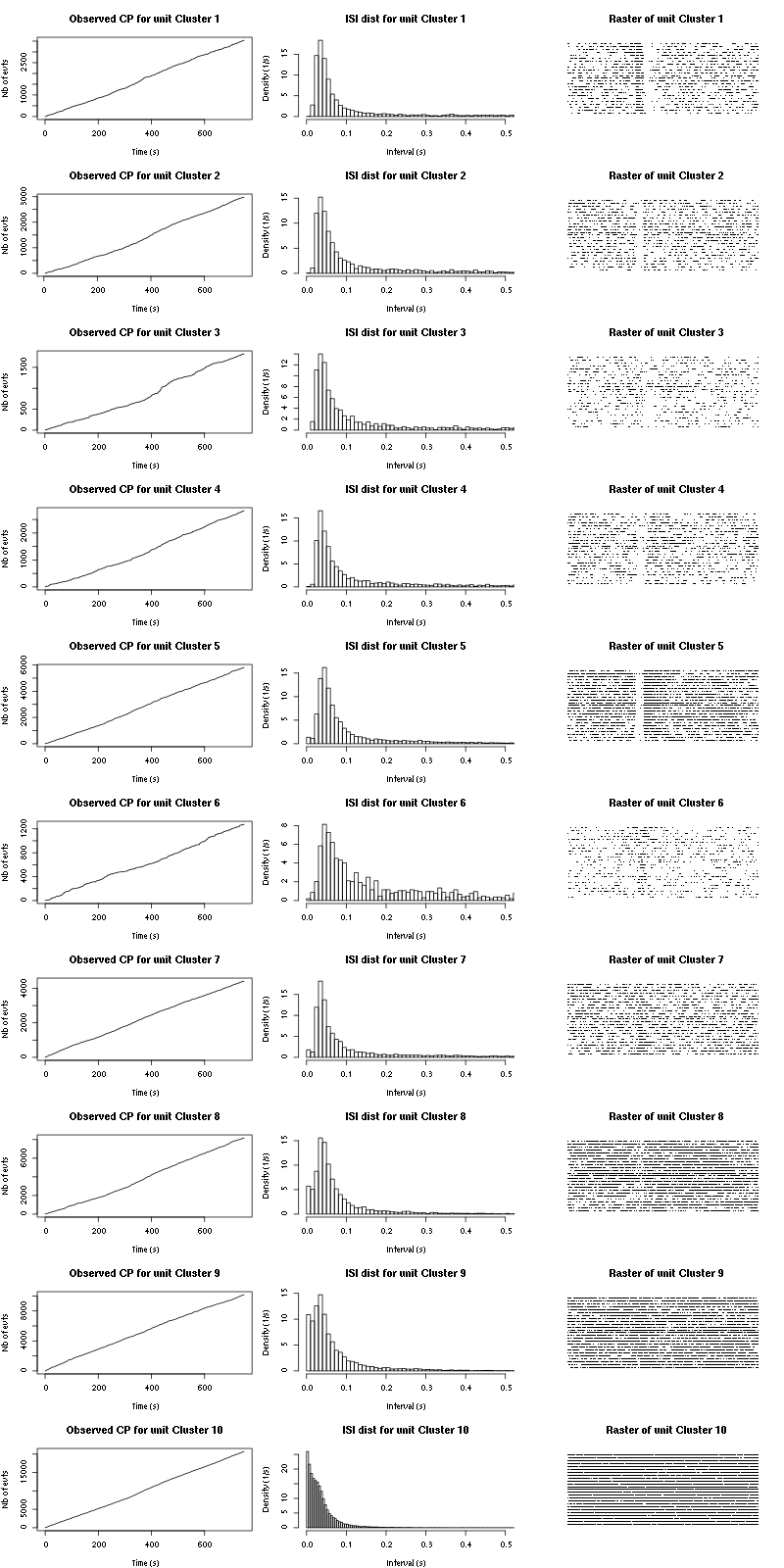
Figure 27: Observed counting processes, empirical inter spike interval distributions and raster plots for Citral.

The BRT and RFT tests give for the first 7 units:

layout_matrix = matrix(0,nr=nbc-3,nc=nbc-3)
counter = 1
for (i in 1:(nbc-3))
    for (j in 1:(nbc-3))
        if (i != j) {
            layout_matrix[i,j] = counter
            counter = counter +1
        }
layout(layout_matrix)
par(mar=c(4,3,4,1))
for (i in 1:(nbc-3))
    for (j in 1:(nbc-3))
        if (i != j)
            test_rt(a_Citral_1_tetB$spike_trains[[i]],
                    a_Citral_1_tetB$spike_trains[[j]],
		    nbins=200,single_trial_duration=30,
                    ylab="",main=paste("Units",i,"and",j))

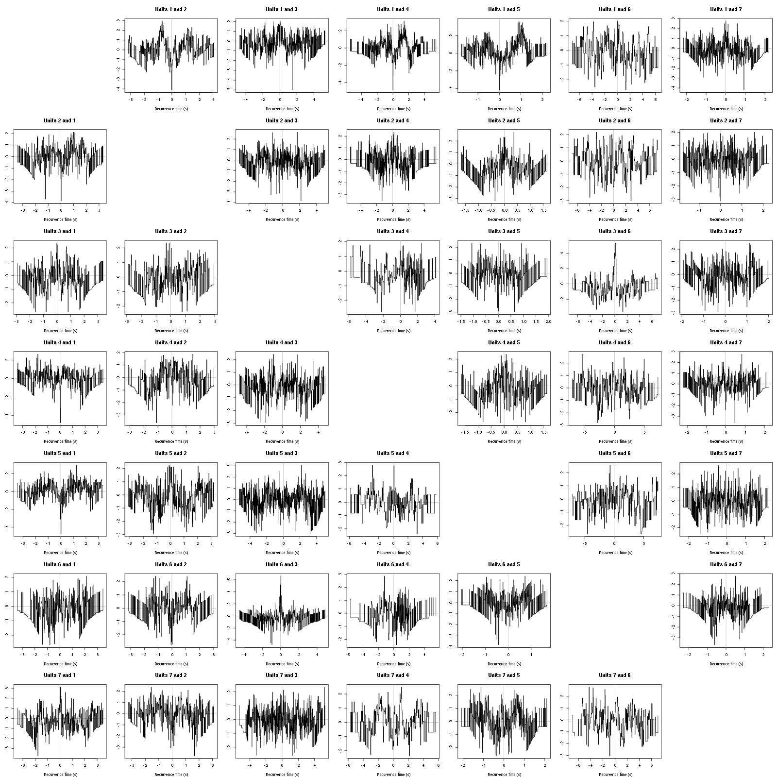
Figure 28: Graphical tests for the first 7 units of the Backward and Forward Reccurrence Times distribution against the null hypothesis (no interaction) during Spontaenous_1. If the null is correct, the curves should be IID draws from a standard normal distribution.

7.3 Save results

Before analyzing the next set of trials we save the output of sort_many_trials to disk with:

save(a_Citral_1_tetB,
     file=paste0("tetB_analysis/tetB_",stim_name,"_summary_obj.rda"))

We write to disk the spike trains in text mode:

for (c_idx in 1:length(a_Citral_1_tetB$spike_trains))
    if (!is.null(a_Citral_1_tetB$spike_trains[[c_idx]]))
        cat(a_Citral_1_tetB$spike_trains[[c_idx]],file=paste0("locust20010214_spike_trains/locust20010214_Citral_tetB_u",c_idx,".txt"),sep="\n")

8 25 trials with `Vanilla`

We will carry out an analysis of the 25 trials from Vanilla_1.

8.1 Do the job

stim_name = "Vanilla_1"
a_Vanilla_1_tetB=sort_many_trials(inter_trial_time=30*15000,
                                 get_data_fct=get_tetrode_data,
                                 stim_name=stim_name,
                                 trial_nbs=1:25,
                                 centers=a_Citral_1_tetB$centers,
                                 counts=a_Citral_1_tetB$counts,
                                 all_at_once_call_list=list(thres=threshold_factor*c(1,1,1,1), 
                                                            filter_length_1=filter_length, filter_length=filter_length, 
                                                            minimalDist_1=15, minimalDist=15, 
                                                            before=c_before, after=c_after, 
                                                            detection_cycle=c(0,0), verbose=1),
                                 layout_matrix=matrix(c(1,1:11),nr=6),new_weight_in_update=0.01
                                 )

8.2 Diagnostic plots

The counts evolution is:

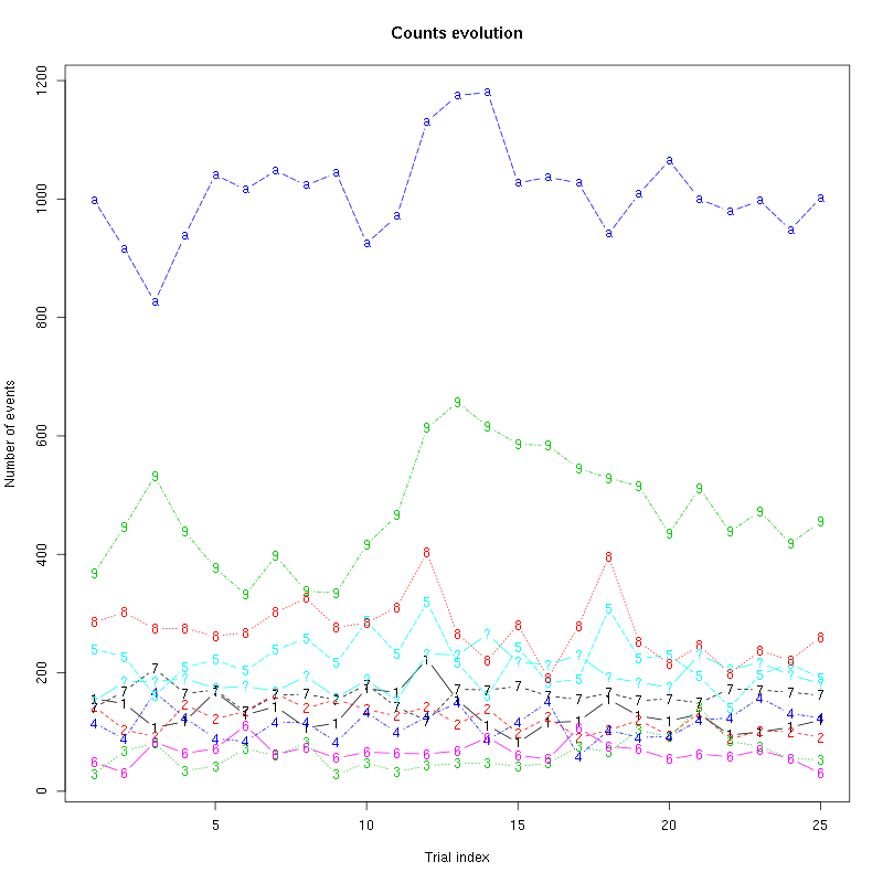
Figure 29: Evolution of the number of events attributed to each unit (1 to 9 and "a") or unclassified ("?") during the 25 trials of Vanilla_1 for tetrodeB.

The waveform evolution is:

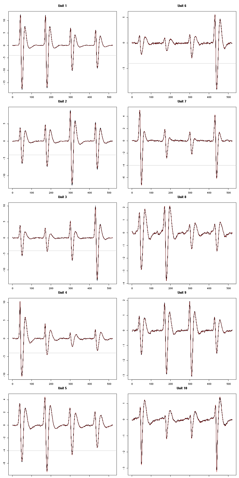
Figure 30: Evolution of the templates of each unit during the 25 trials of Vanilla_1 for tetrodeB.

The observed counting processes, inter spike intervals densities and raster plots are:

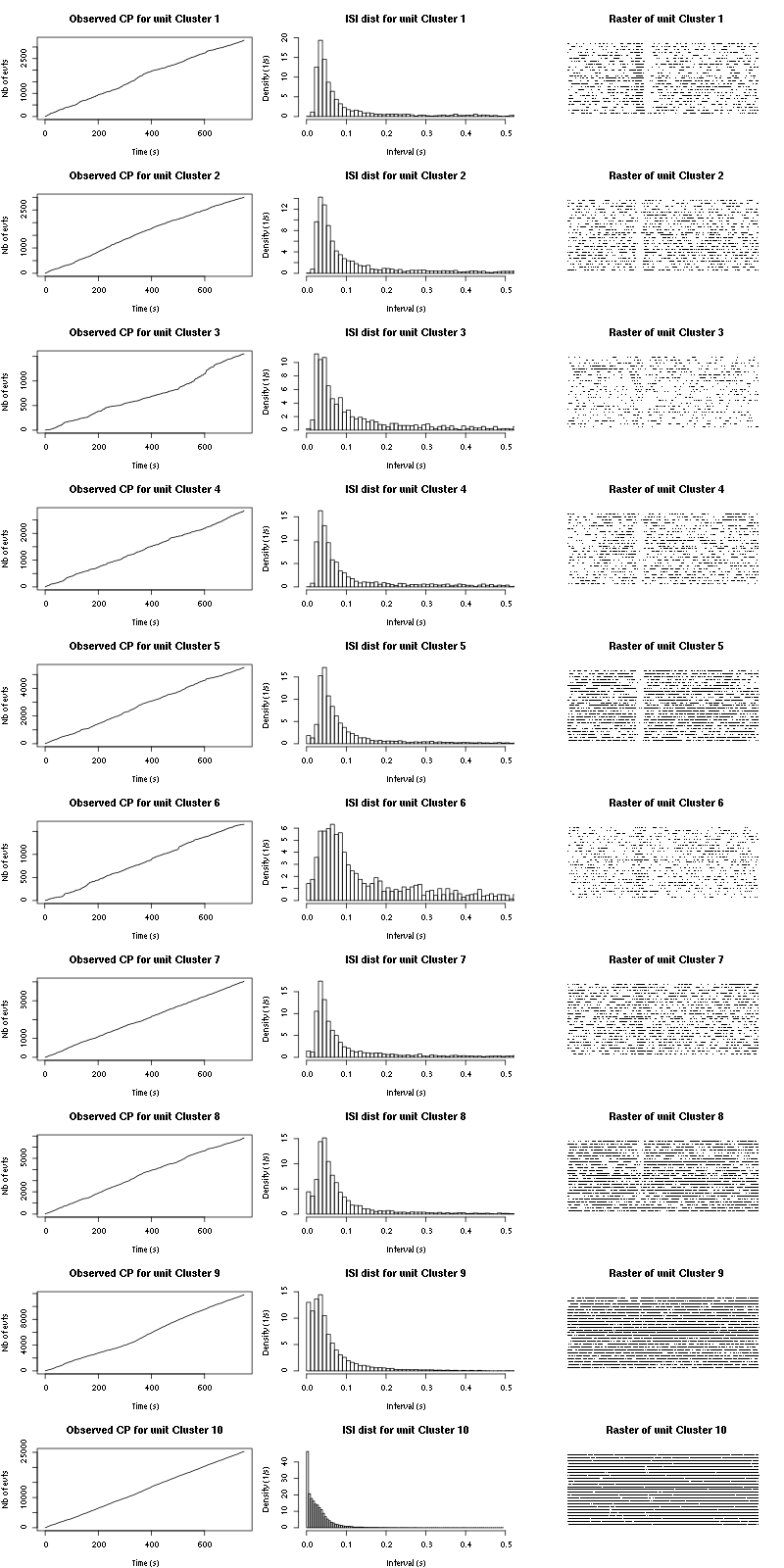
Figure 31: Observed counting processes, empirical inter spike interval distributions and raster plots for Vanilla.

The BRT and RFT tests give for the first 7 units:

layout_matrix = matrix(0,nr=nbc-3,nc=nbc-3)
counter = 1
for (i in 1:(nbc-3))
    for (j in 1:(nbc-3))
        if (i != j) {
            layout_matrix[i,j] = counter
            counter = counter +1
        }
layout(layout_matrix)
par(mar=c(4,3,4,1))
for (i in 1:(nbc-3))
    for (j in 1:(nbc-3))
        if (i != j)
            test_rt(a_Vanilla_1_tetB$spike_trains[[i]],
                    a_Vanilla_1_tetB$spike_trains[[j]],
		    nbins=200,single_trial_duration=30,
                    ylab="",main=paste("Units",i,"and",j))

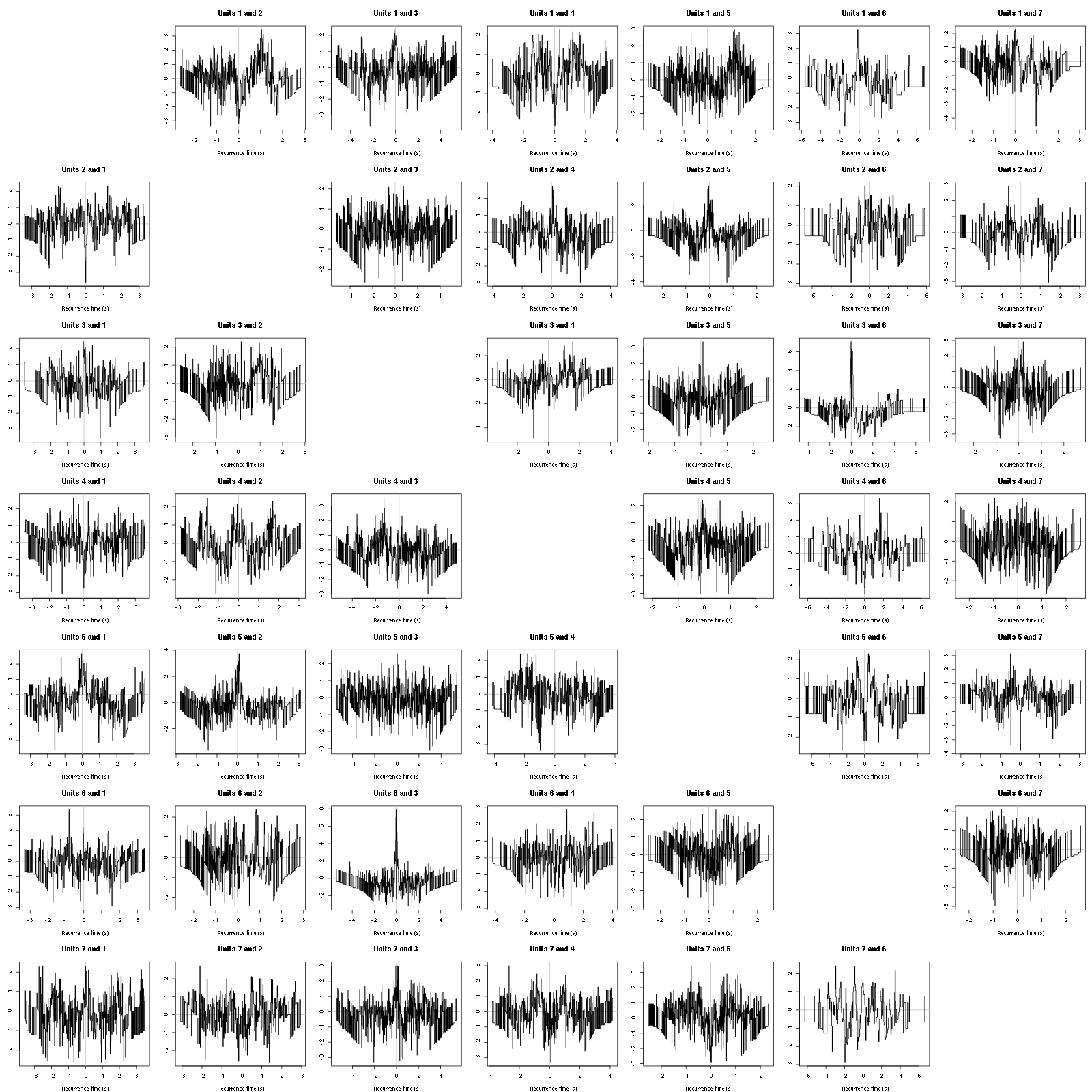
Figure 32: Graphical tests for the first 7 units of the Backward and Forward Reccurrence Times distribution against the null hypothesis (no interaction) during Spontaenous_1. If the null is correct, the curves should be IID draws from a standard normal distribution.

8.3 Save results

Before analyzing the next set of trials we save the output of sort_many_trials to disk with:

save(a_Vanilla_1_tetB,
     file=paste0("tetB_analysis/tetB_",stim_name,"_summary_obj.rda"))

We write to disk the spike trains in text mode:

for (c_idx in 1:length(a_Vanilla_1_tetB$spike_trains))
    if (!is.null(a_Vanilla_1_tetB$spike_trains[[c_idx]]))
        cat(a_Vanilla_1_tetB$spike_trains[[c_idx]],file=paste0("locust20010214_spike_trains/locust20010214_Vanilla_1_tetB_u",c_idx,".txt"),sep="\n")

9 25 trials with `Octanol`

We will carry out an analysis of the 25 trials from Octanol_1. The LabBook mentions the presence of noise in trials 10, 11 and 12, so we skip those.

9.1 Do the job

stim_name = "Octanol_1"
a_Octanol_1_tetB=sort_many_trials(inter_trial_time=30*15000,
                                  get_data_fct=get_tetrode_data,
                                  stim_name=stim_name,
                                  trial_nbs=c(1:9,13:25),
                                  centers=a_Vanilla_1_tetB$centers,
                                  counts=a_Vanilla_1_tetB$counts,
                                  all_at_once_call_list=list(thres=threshold_factor*c(1,1,1,1), 
                                                             filter_length_1=filter_length, filter_length=filter_length, 
                                                             minimalDist_1=15, minimalDist=15, 
                                                             before=c_before, after=c_after, 
                                                             detection_cycle=c(0,0), verbose=1),
                                  layout_matrix=matrix(c(1,1:11),nr=6),new_weight_in_update=0.01
                                  )

9.2 Diagnostic plots

The counts evolution is:

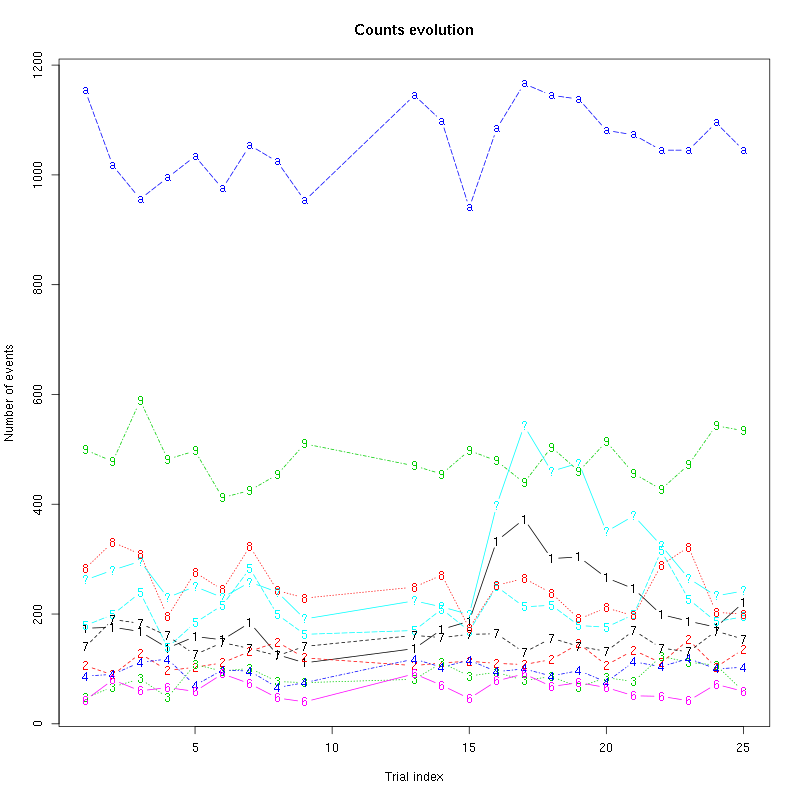
Figure 33: Evolution of the number of events attributed to each unit (1 to 9 and "a") or unclassified ("?") during the 25 trials of Octanol_1 for tetrodeB.

The waveform evolution is:

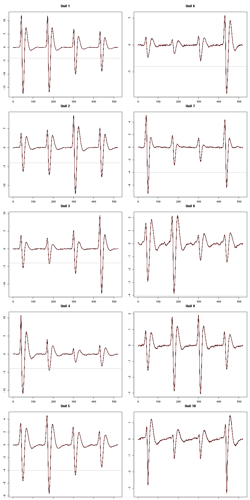
Figure 34: Evolution of the templates of each unit during the 25 trials of Octanol_1 for tetrodeB.

The observed counting processes, inter spike intervals densities and raster plots are:

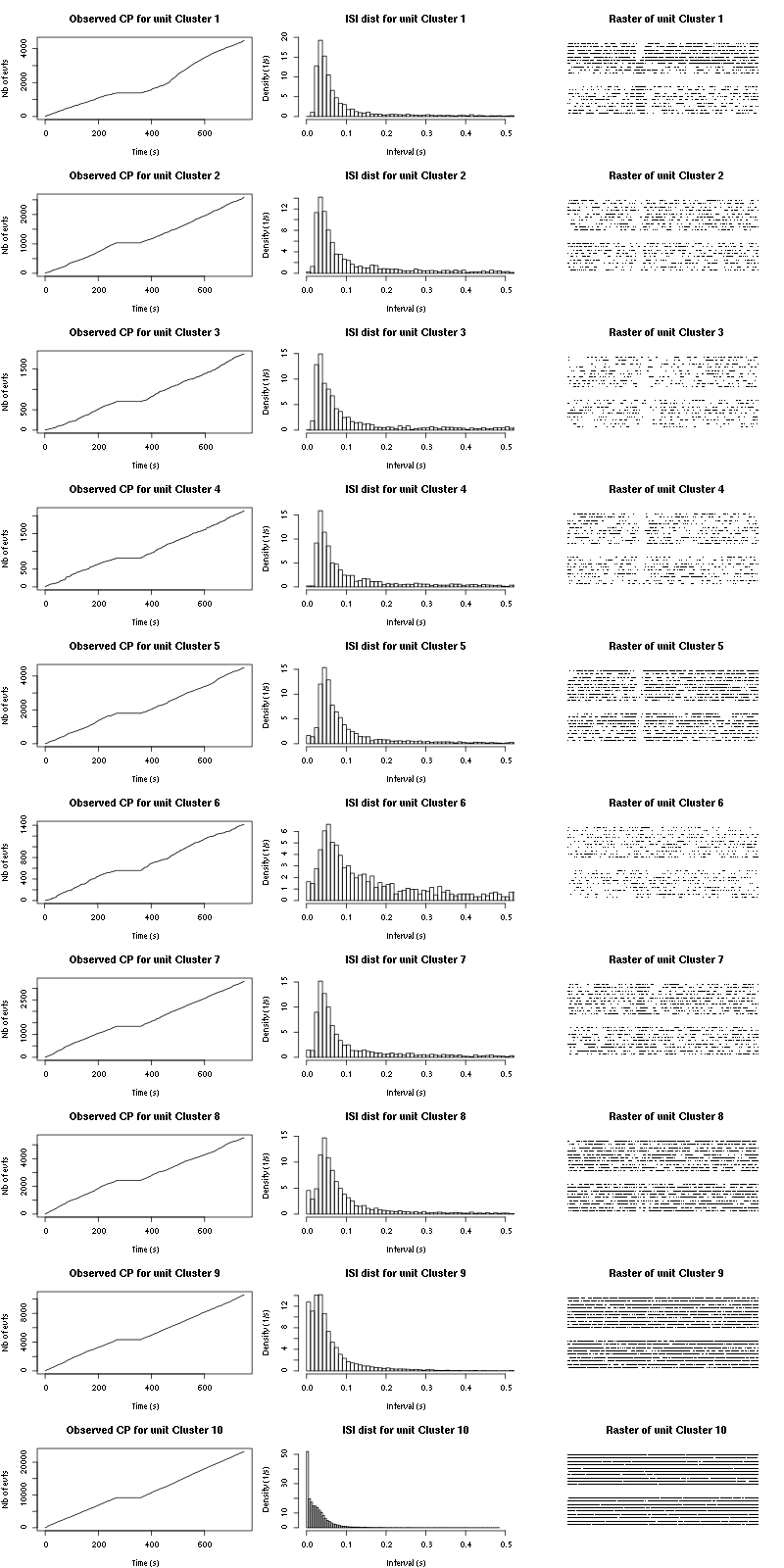
Figure 35: Observed counting processes, empirical inter spike interval distributions and raster plots for Octanol.

The BRT and RFT tests give for the first 7 units:

layout_matrix = matrix(0,nr=nbc-3,nc=nbc-3)
counter = 1
for (i in 1:(nbc-3))
    for (j in 1:(nbc-3))
        if (i != j) {
            layout_matrix[i,j] = counter
            counter = counter +1
        }
layout(layout_matrix)
par(mar=c(4,3,4,1))
for (i in 1:(nbc-3))
    for (j in 1:(nbc-3))
        if (i != j)
            test_rt(a_Octanol_1_tetB$spike_trains[[i]],
                    a_Octanol_1_tetB$spike_trains[[j]],
		    nbins=200,single_trial_duration=30,
                    ylab="",main=paste("Units",i,"and",j))

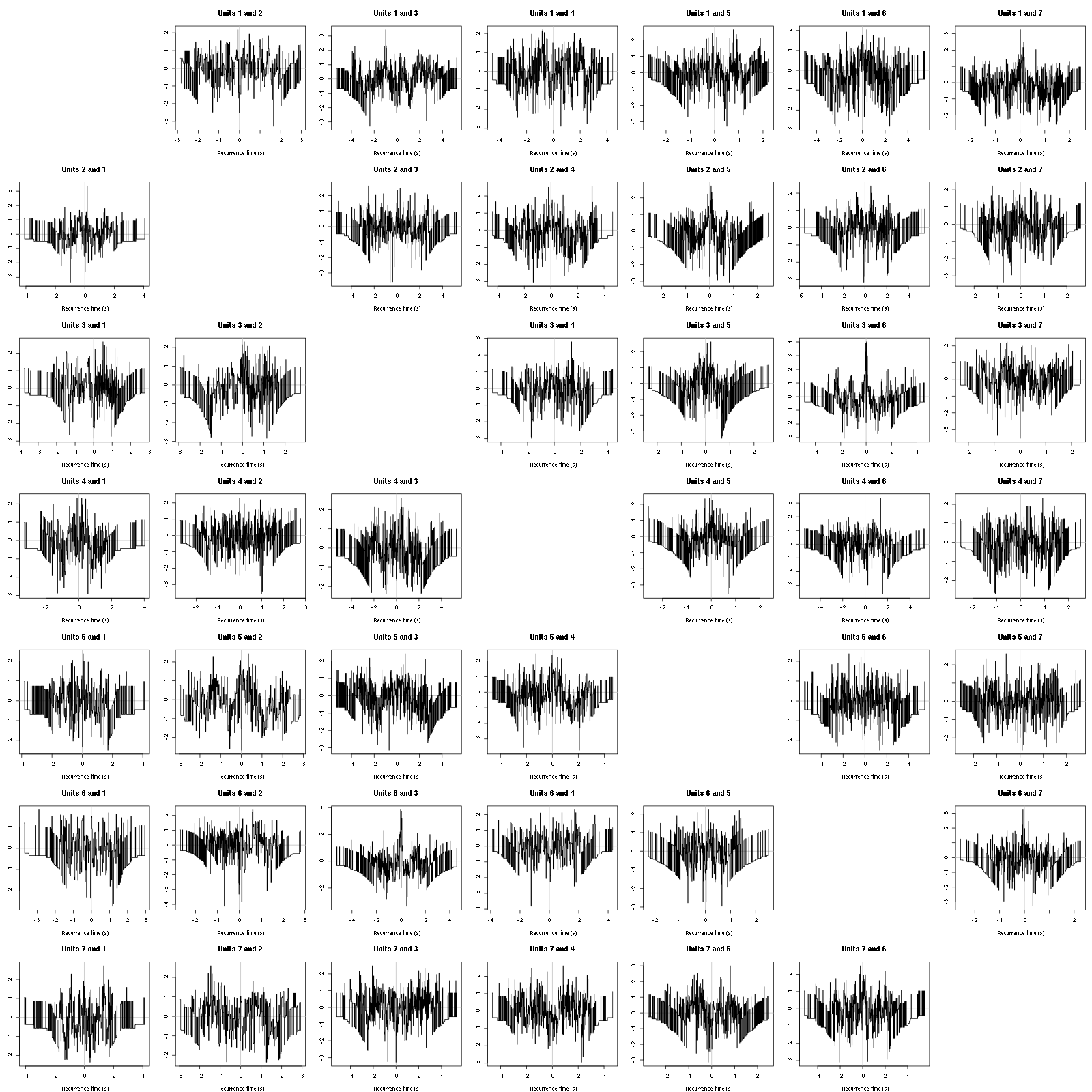
Figure 36: Graphical tests for the first 7 units of the Backward and Forward Reccurrence Times distribution against the null hypothesis (no interaction) during Spontaenous_1. If the null is correct, the curves should be IID draws from a standard normal distribution.

9.3 Save results

Before analyzing the next set of trials we save the output of sort_many_trials to disk with:

save(a_Octanol_1_tetB,
     file=paste0("tetB_analysis/tetB_",stim_name,"_summary_obj.rda"))

We write to disk the spike trains in text mode:

for (c_idx in 1:length(a_Octanol_1_tetB$spike_trains))
    if (!is.null(a_Octanol_1_tetB$spike_trains[[c_idx]]))
        cat(a_Octanol_1_tetB$spike_trains[[c_idx]],file=paste0("locust20010214_spike_trains/locust20010214_Octanol_1_tetB_u",c_idx,".txt"),sep="\n")

10 25 trials with `Mint`

We will carry out an analysis of the 25 trials from Mint_1.

10.1 Do the job

stim_name = "Mint_1"
a_Mint_1_tetB=sort_many_trials(inter_trial_time=30*15000,
                               get_data_fct=get_tetrode_data,
                               stim_name=stim_name,
                               trial_nbs=1:25,
                               centers=a_Octanol_1_tetB$centers,
                               counts=a_Octanol_1_tetB$counts,
                               all_at_once_call_list=list(thres=threshold_factor*c(1,1,1,1), 
                                                          filter_length_1=filter_length, filter_length=filter_length, 
                                                          minimalDist_1=15, minimalDist=15, 
                                                          before=c_before, after=c_after, 
                                                          detection_cycle=c(0,0), verbose=1),
                               layout_matrix=matrix(c(1,1:11),nr=6),new_weight_in_update=0.01
                               )

10.2 Diagnostic plots

The counts evolution is:

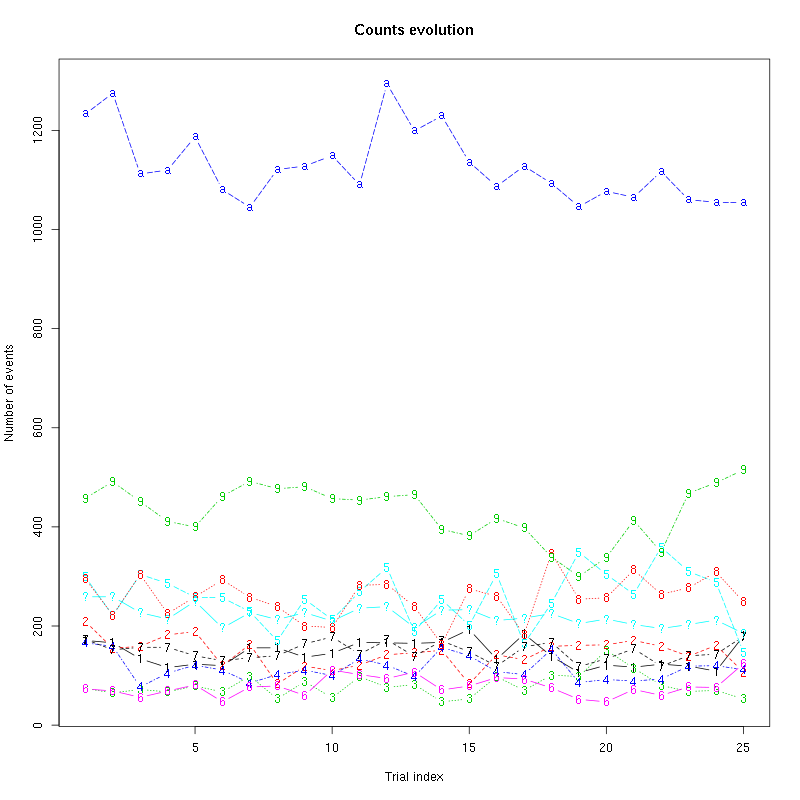
Figure 37: Evolution of the number of events attributed to each unit (1 to 9 and "a") or unclassified ("?") during the 25 trials of Mint_1 for tetrodeB.

The waveform evolution is:

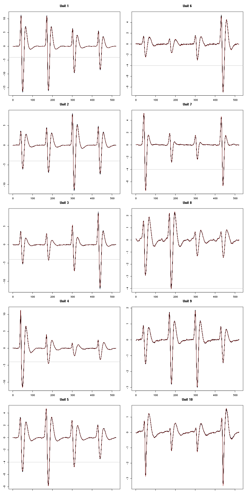
Figure 38: Evolution of the templates of each unit during the 25 trials of Mint_1 for tetrodeB.

The observed counting processes, inter spike intervals densities and raster plots are:

Figure 39: Observed counting processes, empirical inter spike interval distributions and raster plots for Mint.

The BRT and RFT tests give for the first 7 units:

layout_matrix = matrix(0,nr=nbc-3,nc=nbc-3)
counter = 1
for (i in 1:(nbc-3))
    for (j in 1:(nbc-3))
        if (i != j) {
            layout_matrix[i,j] = counter
            counter = counter +1
        }
layout(layout_matrix)
par(mar=c(4,3,4,1))
for (i in 1:(nbc-3))
    for (j in 1:(nbc-3))
        if (i != j)
            test_rt(a_Mint_1_tetB$spike_trains[[i]],
                    a_Mint_1_tetB$spike_trains[[j]],
		    nbins=200,single_trial_duration=30,
                    ylab="",main=paste("Units",i,"and",j))

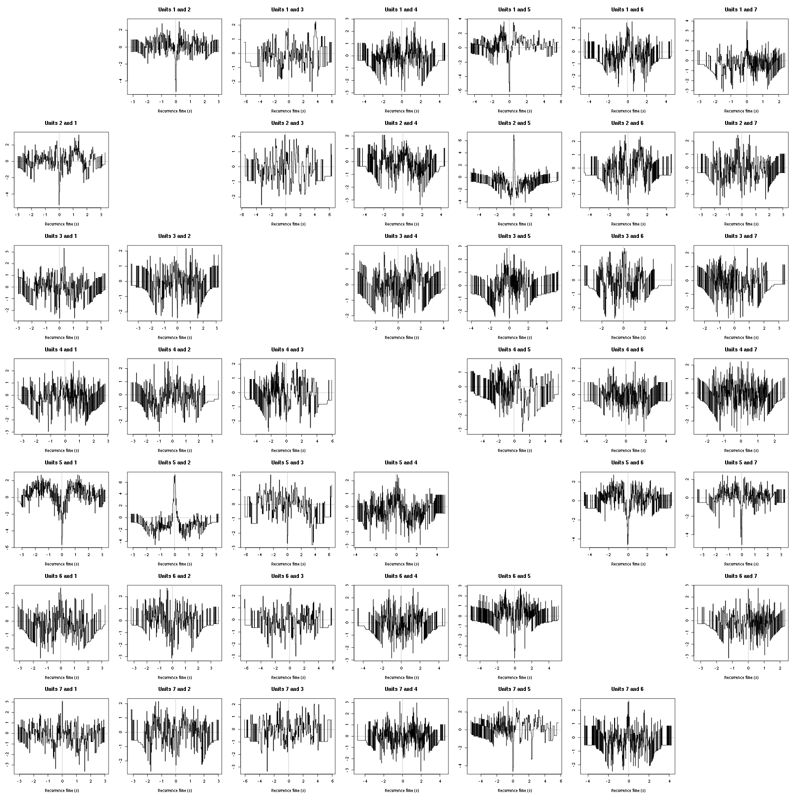
Figure 40: Graphical tests for the first 7 units of the Backward and Forward Reccurrence Times distribution against the null hypothesis (no interaction) during Spontaenous_1. If the null is correct, the curves should be IID draws from a standard normal distribution.

10.3 Save results

Before analyzing the next set of trials we save the output of sort_many_trials to disk with:

save(a_Mint_1_tetB,
     file=paste0("tetB_analysis/tetB_",stim_name,"_summary_obj.rda"))

We write to disk the spike trains in text mode:

for (c_idx in 1:length(a_Mint_1_tetB$spike_trains))
    if (!is.null(a_Mint_1_tetB$spike_trains[[c_idx]]))
        cat(a_Mint_1_tetB$spike_trains[[c_idx]],file=paste0("locust20010214_spike_trains/locust20010214_Mint_1_tetB_u",c_idx,".txt"),sep="\n")

11 25 trials with `C3H_2`

We will carry out an analysis of the second set of 25 trials with Cis-3-Hexen-1-ol from C3H_2.

11.1 Do the job

stim_name = "C3H_2"
a_C3H_2_tetB=sort_many_trials(inter_trial_time=30*15000,
                              get_data_fct=get_tetrode_data,
                              stim_name=stim_name,
                              trial_nbs=1:25,
                              centers=a_Mint_1_tetB$centers,
                              counts=a_Mint_1_tetB$counts,
                              all_at_once_call_list=list(thres=threshold_factor*c(1,1,1,1), 
                                                         filter_length_1=filter_length, filter_length=filter_length, 
                                                         minimalDist_1=15, minimalDist=15, 
                                                         before=c_before, after=c_after, 
                                                         detection_cycle=c(0,0), verbose=1),
                              layout_matrix=matrix(c(1,1:11),nr=6),new_weight_in_update=0.01
                              )

11.2 Diagnostic plots

The counts evolution is:

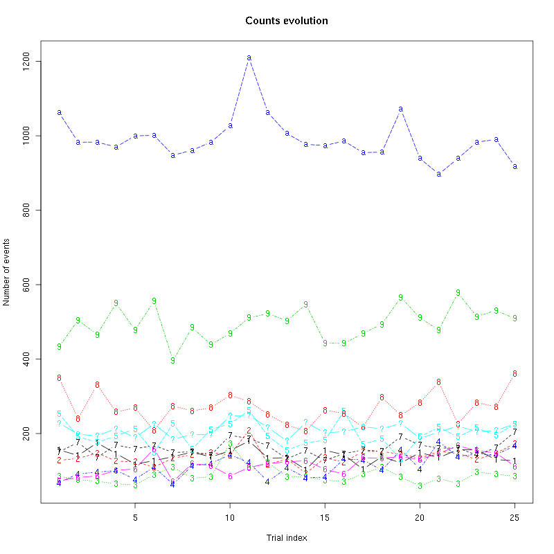
Figure 41: Evolution of the number of events attributed to each unit (1 to 9 and "a") or unclassified ("?") during the 25 trials of C3H_2 for tetrodeB.

The waveform evolution is:

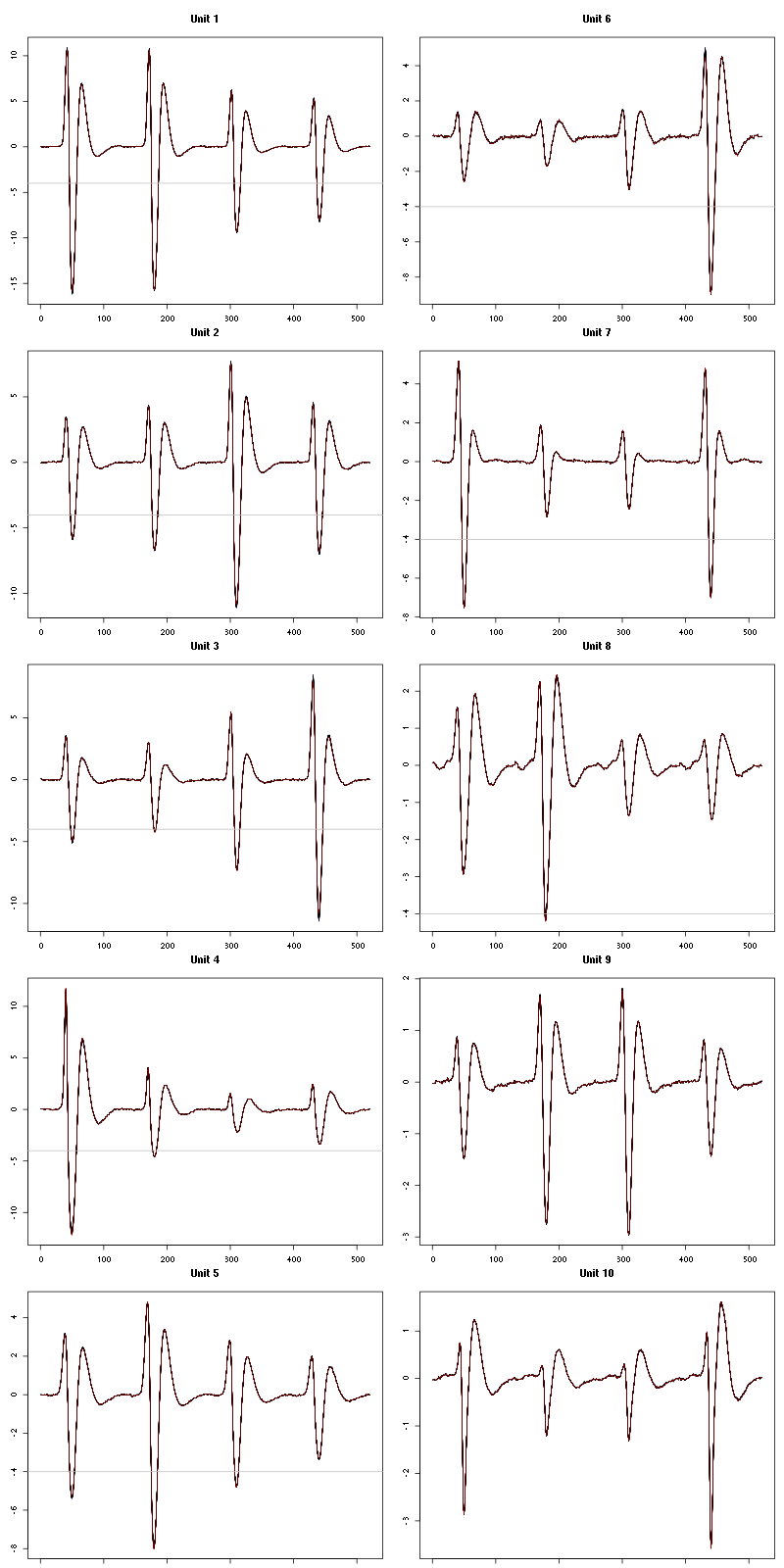
Figure 42: Evolution of the templates of each unit during the 25 trials of C3H_2 for tetrodeB.

The observed counting processes, inter spike intervals densities and raster plots are:

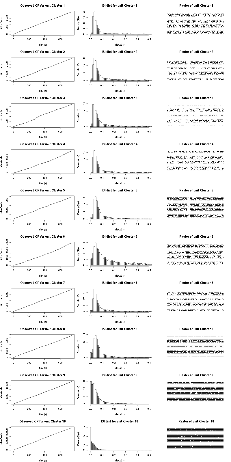
Figure 43: Observed counting processes, empirical inter spike interval distributions and raster plots for Mint.

The BRT and RFT tests give for the first 7 units:

layout_matrix = matrix(0,nr=nbc-3,nc=nbc-3)
counter = 1
for (i in 1:(nbc-3))
    for (j in 1:(nbc-3))
        if (i != j) {
            layout_matrix[i,j] = counter
            counter = counter +1
        }
layout(layout_matrix)
par(mar=c(4,3,4,1))
for (i in 1:(nbc-3))
    for (j in 1:(nbc-3))
        if (i != j)
            test_rt(a_C3H_2_tetB$spike_trains[[i]],
                    a_C3H_2_tetB$spike_trains[[j]],
		    nbins=200,single_trial_duration=30,
                    ylab="",main=paste("Units",i,"and",j))

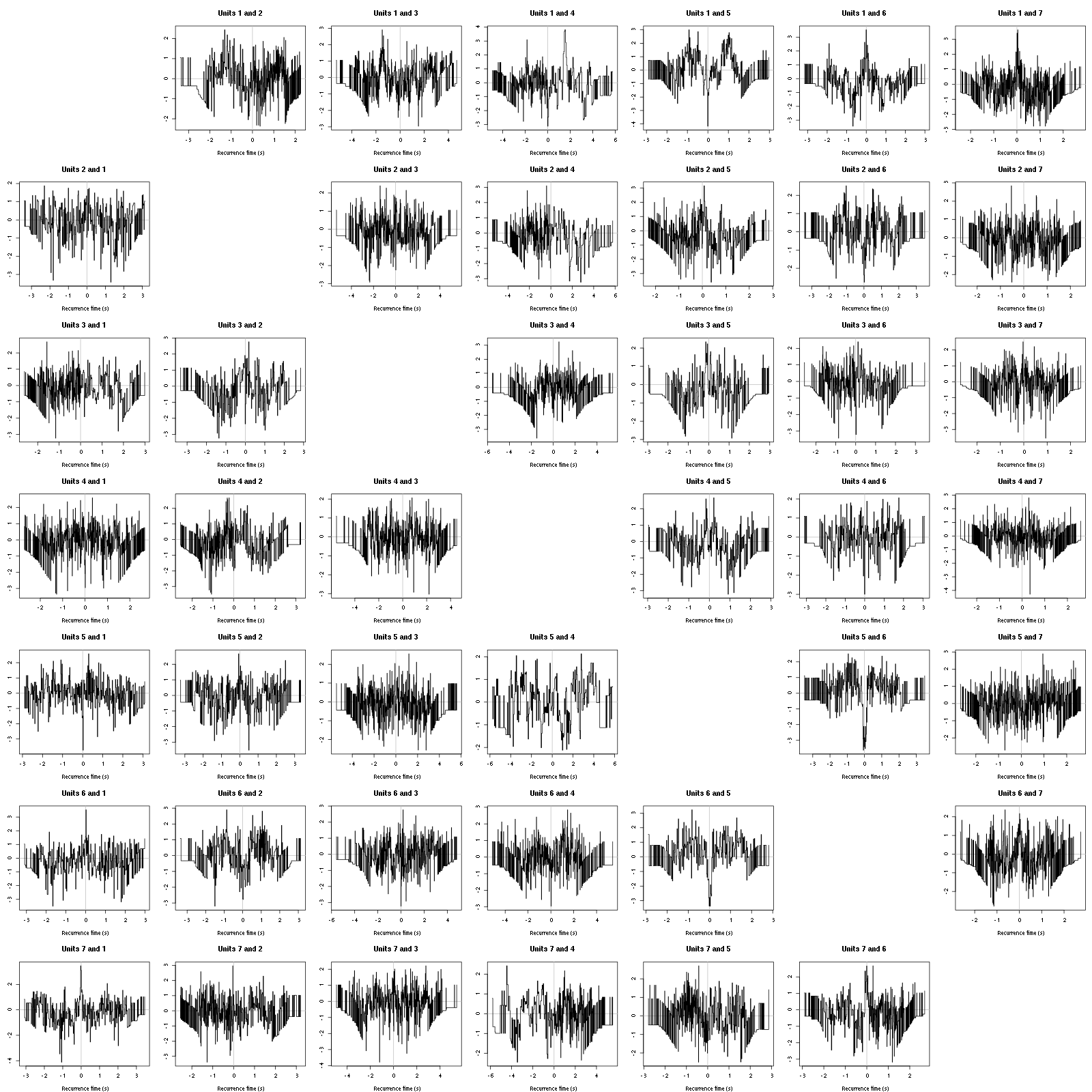
Figure 44: Graphical tests for the first 7 units of the Backward and Forward Reccurrence Times distribution against the null hypothesis (no interaction) during Spontaenous_1. If the null is correct, the curves should be IID draws from a standard normal distribution.

11.3 Save results

Before analyzing the next set of trials we save the output of sort_many_trials to disk with:

save(a_C3H_2_tetB,
     file=paste0("tetB_analysis/tetB_",stim_name,"_summary_obj.rda"))

We write to disk the spike trains in text mode:

for (c_idx in 1:length(a_C3H_2_tetB$spike_trains))
    if (!is.null(a_C3H_2_tetB$spike_trains[[c_idx]]))
        cat(a_C3H_2_tetB$spike_trains[[c_idx]],file=paste0("locust20010214_spike_trains/locust20010214_C3H_2_tetB_u",c_idx,".txt"),sep="\n")

12 30 trials of `Spontaneous_3`

We must redefine our get_tetrode_data function since the HDF5 containing the data is not the one where the previous data were stored:

12.1 Redefine `get_tetrode_data`

get_tetrode_data = function(trial_idx,stim="Spontaneous_1") {
    prefix = ifelse(trial_idx<10,
                    paste0("/",stim,"/trial_0",trial_idx),
                    paste0("/",stim,"/trial_",trial_idx)
                    )
    cbind(h5read("locust20010214_part2.hdf5", paste0(prefix,"/ch02")),
          h5read("locust20010214_part2.hdf5", paste0(prefix,"/ch03")),
          h5read("locust20010214_part2.hdf5", paste0(prefix,"/ch05")),
          h5read("locust20010214_part2.hdf5", paste0(prefix,"/ch07")))
}

12.2 Do the job

stim_name = "Spontaneous_3"
a_Spontaneous_3_tetB=sort_many_trials(inter_trial_time=30*15000,
                                      get_data_fct=get_tetrode_data,
                                      stim_name=stim_name,
                                      trial_nbs=1:30,
                                      centers=a_C3H_2_tetB$centers,
                                      counts=a_C3H_2_tetB$counts,
                                      all_at_once_call_list=list(thres=threshold_factor*c(1,1,1,1), 
                                                                 filter_length_1=filter_length, filter_length=filter_length, 
                                                                 minimalDist_1=15, minimalDist=15, 
                                                                 before=c_before, after=c_after, 
                                                                 detection_cycle=c(0,0), verbose=1),
                                      layout_matrix=matrix(c(1,1:11),nr=6),new_weight_in_update=0.01
                                      )

12.3 Diagnostic plots

The counts evolution is:

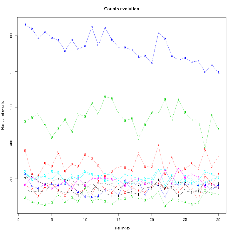
Figure 45: Evolution of the number of events attributed to each unit (1 to 9 and "a") or unclassified ("?") during the 30 trials of Spontaneous_3 for tetrodeB.

The waveform evolution is:

Figure 46: Evolution of the templates of each unit during the 30 trials of Spontaneous_3 for tetrodeB.

The observed counting processes and inter spike intervals densities are:

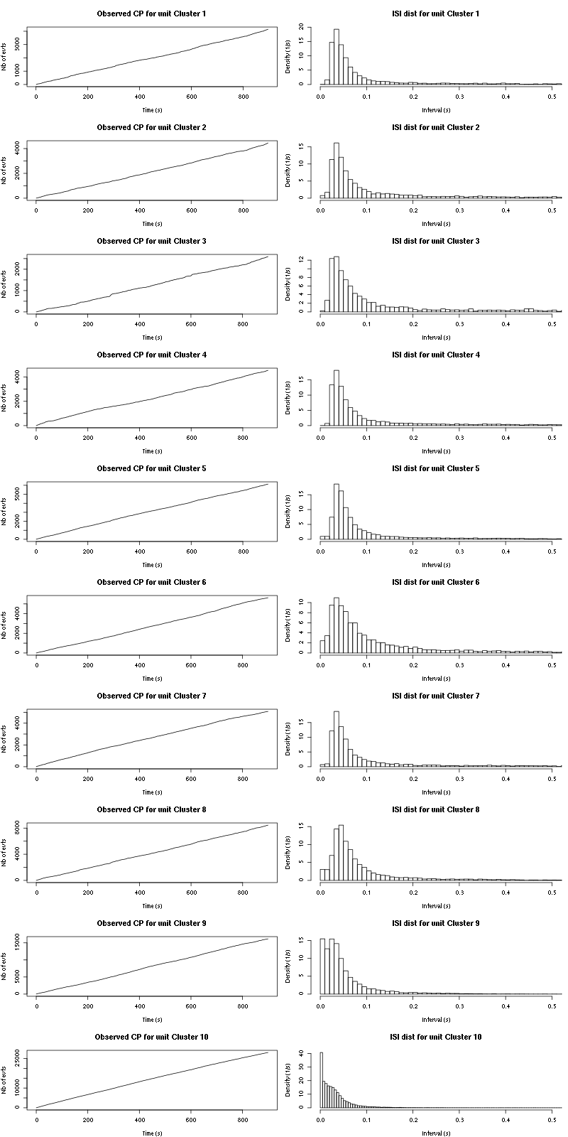
Figure 47: Observed counting processes, empirical inter spike interval distributions and raster plots for Spontaneous_3.

The BRT and RFT tests give for the first 7 units:

layout_matrix = matrix(0,nr=nbc-3,nc=nbc-3)
counter = 1
for (i in 1:(nbc-3))
    for (j in 1:(nbc-3))
        if (i != j) {
            layout_matrix[i,j] = counter
            counter = counter +1
        }
layout(layout_matrix)
par(mar=c(4,3,4,1))
for (i in 1:(nbc-3))
    for (j in 1:(nbc-3))
        if (i != j)
            test_rt(a_Spontaneous_3_tetB$spike_trains[[i]],
                    a_Spontaneous_3_tetB$spike_trains[[j]],
		    nbins=200,single_trial_duration=30,
                    ylab="",main=paste("Units",i,"and",j))

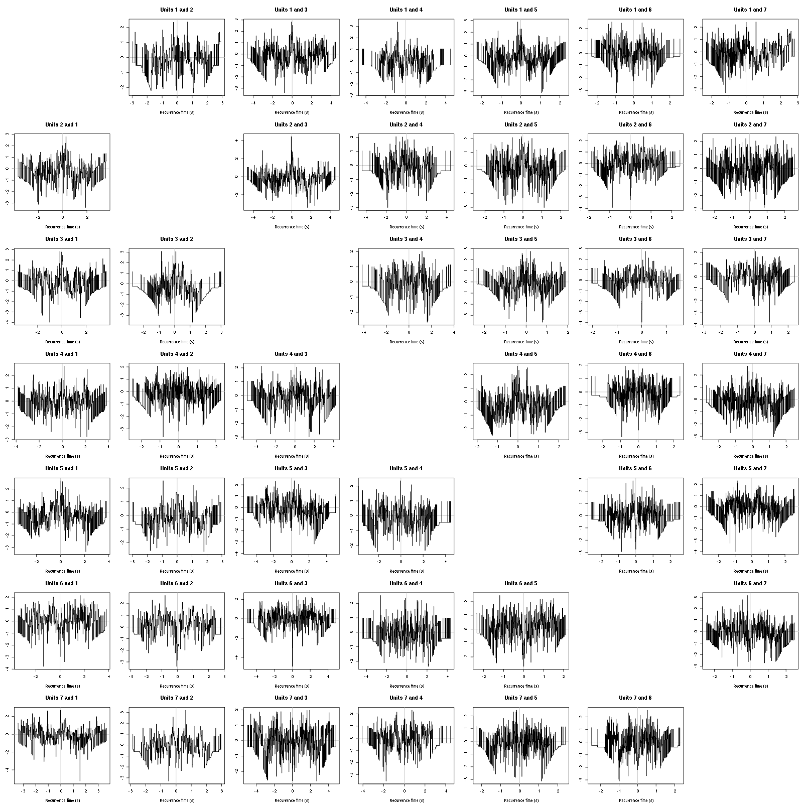
Figure 48: Graphical tests for the first 7 units of the Backward and Forward Reccurrence Times distribution against the null hypothesis (no interaction) during Spontaenous_1. If the null is correct, the curves should be IID draws from a standard normal distribution.

12.4 Save results

Before analyzing the next set of trials we save the output of sort_many_trials to disk with:

save(a_Spontaneous_3_tetB,
     file=paste0("tetB_analysis/tetB_",stim_name,"_summary_obj.rda"))

We write to disk the spike trains in text mode:

for (c_idx in 1:length(a_Spontaneous_3_tetB$spike_trains))
    if (!is.null(a_Spontaneous_3_tetB$spike_trains[[c_idx]]))
        cat(a_Spontaneous_3_tetB$spike_trains[[c_idx]],file=paste0("locust20010214_spike_trains/locust20010214_Spontaneous_3_tetB_u",c_idx,".txt"),sep="\n")

13 30 trials of `Spontaneous_4`

We now analyze the 30 trials from Spontaneous_4.

13.1 Do the job

stim_name = "Spontaneous_4"
a_Spontaneous_4_tetB=sort_many_trials(inter_trial_time=30*15000,
                                      get_data_fct=get_tetrode_data,
                                      stim_name=stim_name,
                                      trial_nbs=1:30,
                                      centers=a_Spontaneous_3_tetB$centers,
                                      counts=a_Spontaneous_3_tetB$counts,
                                      all_at_once_call_list=list(thres=threshold_factor*c(1,1,1,1), 
                                                                 filter_length_1=filter_length, filter_length=filter_length, 
                                                                 minimalDist_1=15, minimalDist=15, 
                                                                 before=c_before, after=c_after, 
                                                                 detection_cycle=c(0,0), verbose=1),
                                      layout_matrix=matrix(c(1,1:11),nr=6),new_weight_in_update=0.01
                                      )

13.2 Diagnostic plots

The counts evolution is:

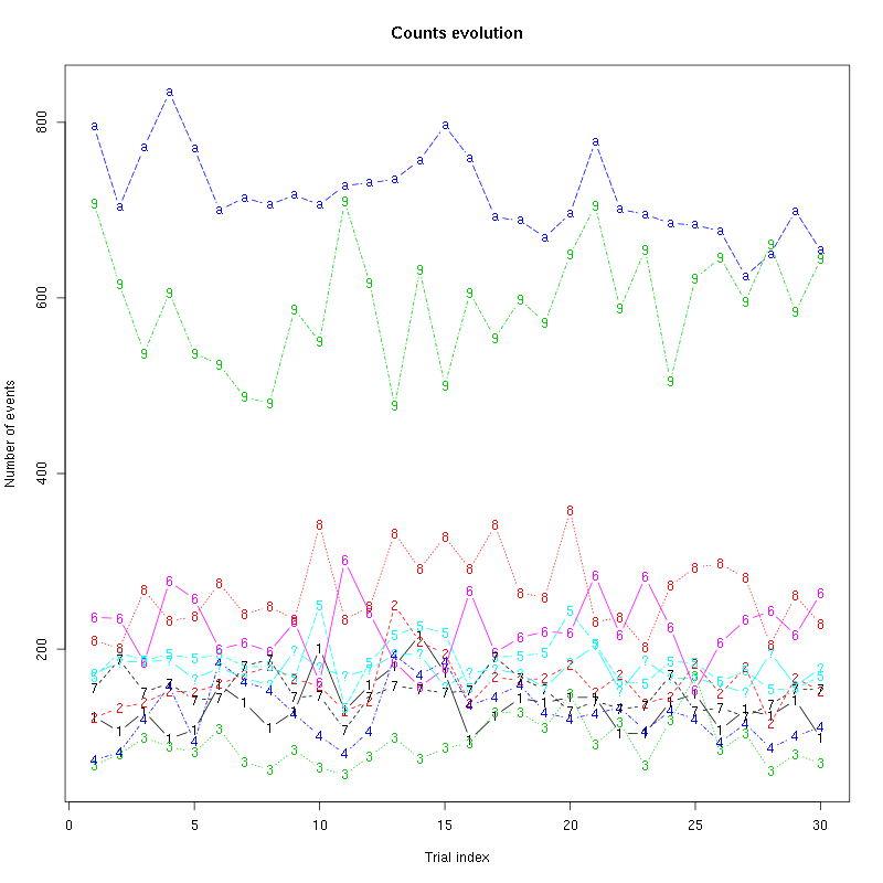
Figure 49: Evolution of the number of events attributed to each unit (1 to 9 and "a") or unclassified ("?") during the 30 trials of Spontaneous_4 for tetrodeB.

The waveform evolution is:

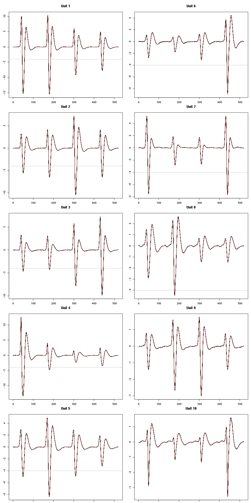
Figure 50: Evolution of the templates of each unit during the 30 trials of Spontaneous_4 for tetrodeB.

The observed counting processes and inter spike intervals densities are:

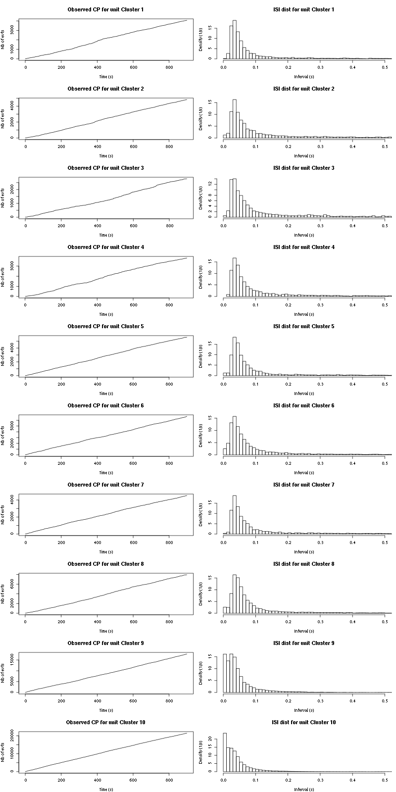
Figure 51: Observed counting processes, empirical inter spike interval distributions and raster plots for Spontaneous_4.

The BRT and RFT tests give for the first 7 units:

layout_matrix = matrix(0,nr=nbc-3,nc=nbc-3)
counter = 1
for (i in 1:(nbc-3))
    for (j in 1:(nbc-3))
        if (i != j) {
            layout_matrix[i,j] = counter
            counter = counter +1
        }
layout(layout_matrix)
par(mar=c(4,3,4,1))
for (i in 1:(nbc-3))
    for (j in 1:(nbc-3))
        if (i != j)
            test_rt(a_Spontaneous_4_tetB$spike_trains[[i]],
                    a_Spontaneous_4_tetB$spike_trains[[j]],
		    nbins=200,single_trial_duration=30,
                    ylab="",main=paste("Units",i,"and",j))

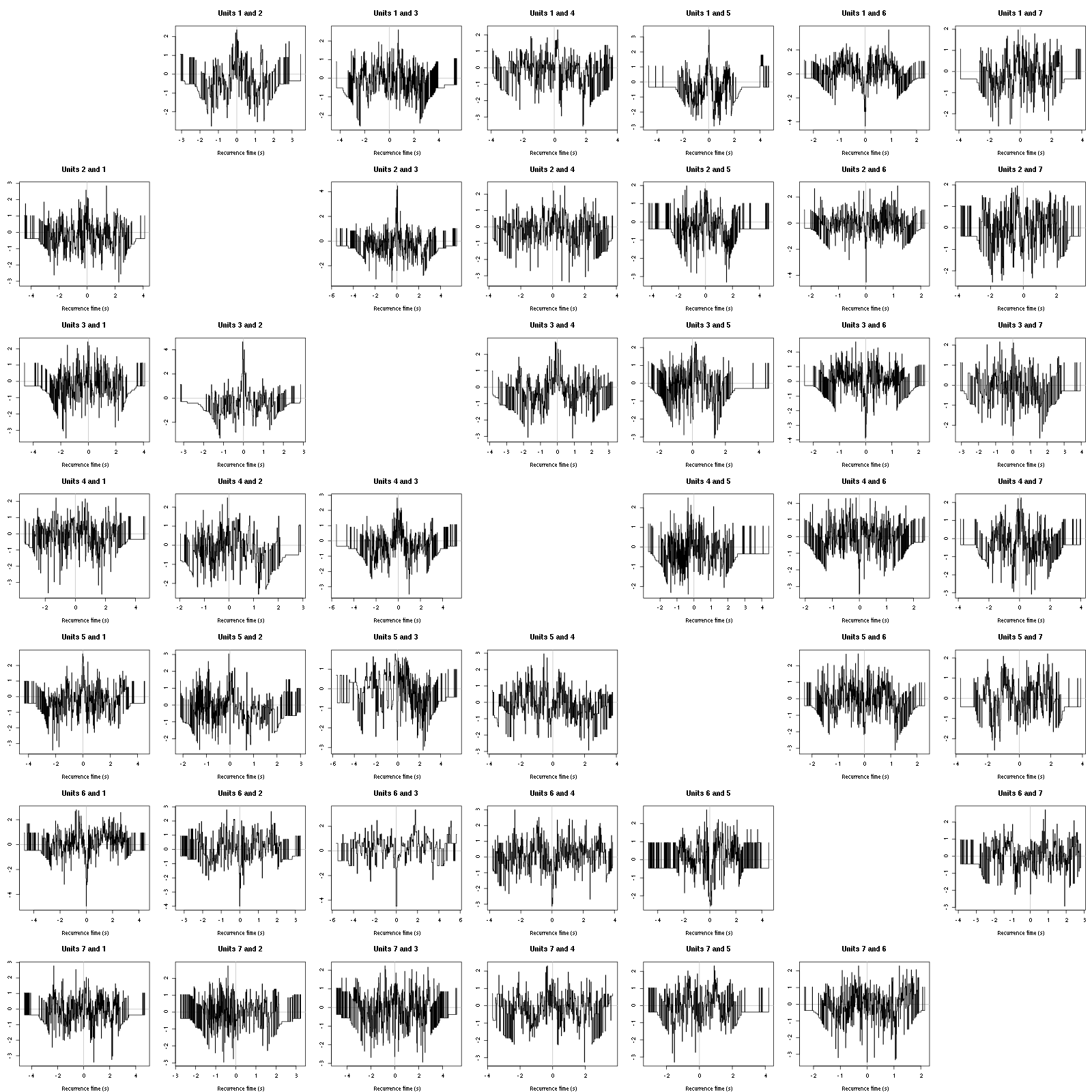
Figure 52: Graphical tests for the first 7 units of the Backward and Forward Reccurrence Times distribution against the null hypothesis (no interaction) during Spontaenous_1. If the null is correct, the curves should be IID draws from a standard normal distribution.

13.3 Save results

Before analyzing the next set of trials we save the output of sort_many_trials to disk with:

save(a_Spontaneous_4_tetB,
     file=paste0("tetB_analysis/tetB_",stim_name,"_summary_obj.rda"))

We write to disk the spike trains in text mode:

for (c_idx in 1:length(a_Spontaneous_4_tetB$spike_trains))
    if (!is.null(a_Spontaneous_4_tetB$spike_trains[[c_idx]]))
        cat(a_Spontaneous_4_tetB$spike_trains[[c_idx]],file=paste0("locust20010214_spike_trains/locust20010214_Spontaneous_4_tetB_u",c_idx,".txt"),sep="\n")

14 30 trials of `C3H_3`

14.1 Do the job

stim_name = "C3H_3"
a_C3H_3_tetB=sort_many_trials(inter_trial_time=30*15000,
                              get_data_fct=get_tetrode_data,
                              stim_name=stim_name,
                              trial_nbs=1:30,
                              centers=a_Spontaneous_4_tetB$centers,
                              counts=a_Spontaneous_4_tetB$counts,
                              all_at_once_call_list=list(thres=threshold_factor*c(1,1,1,1), 
                                                         filter_length_1=filter_length, filter_length=filter_length, 
                                                         minimalDist_1=15, minimalDist=15, 
                                                         before=c_before, after=c_after, 
                                                         detection_cycle=c(0,0), verbose=1),
                              layout_matrix=matrix(c(1,1:11),nr=6),new_weight_in_update=0.01
                              )

14.2 Diagnostic plots

The counts evolution is:

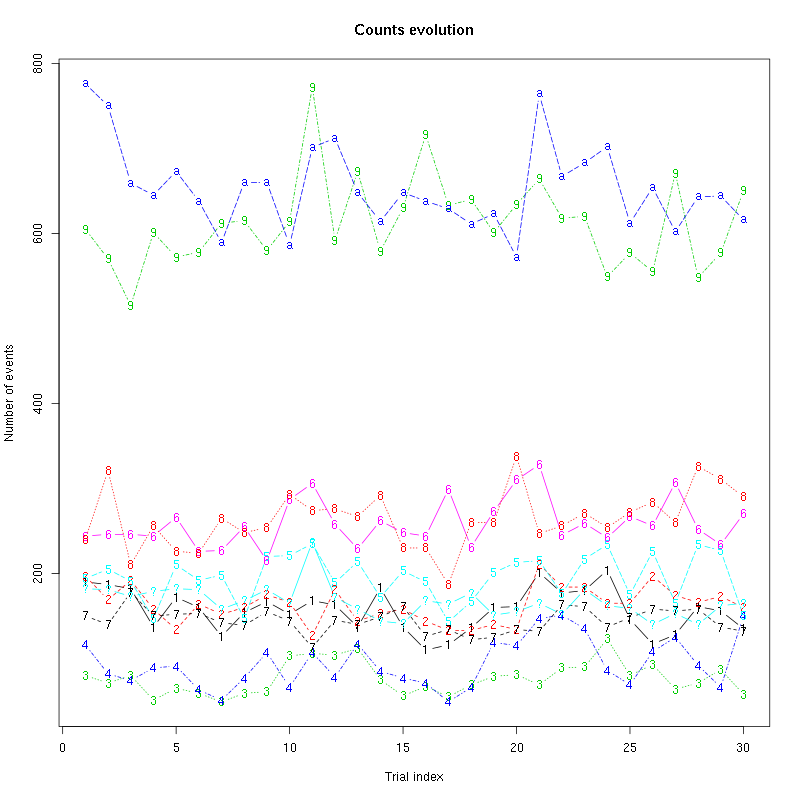
Figure 53: Evolution of the number of events attributed to each unit (1 to 9 and "a") or unclassified ("?") during the 30 trials of C3H_3 for tetrodeB.

The waveform evolution is:

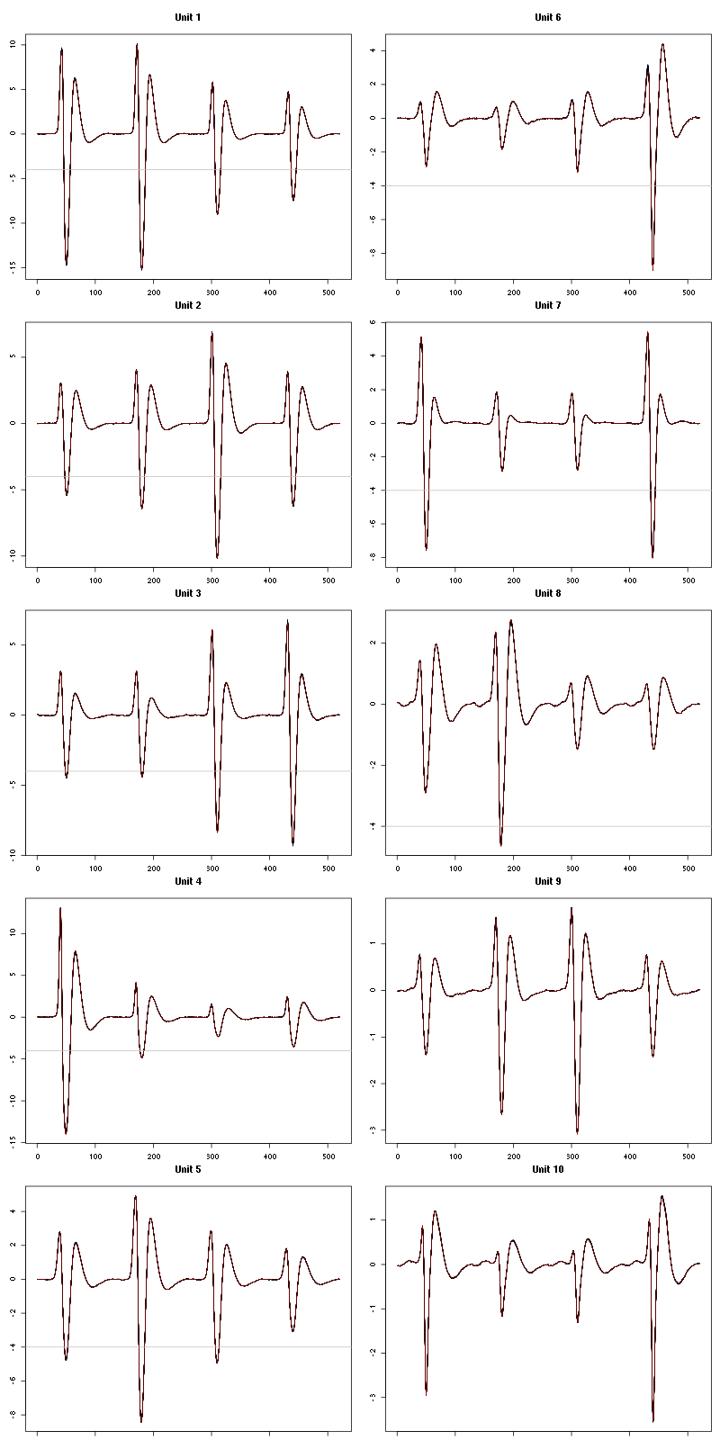
Figure 54: Evolution of the templates of each unit during the 30 trials of C3H_3 for tetrodeB.

The observed counting processes and inter spike intervals densities are:

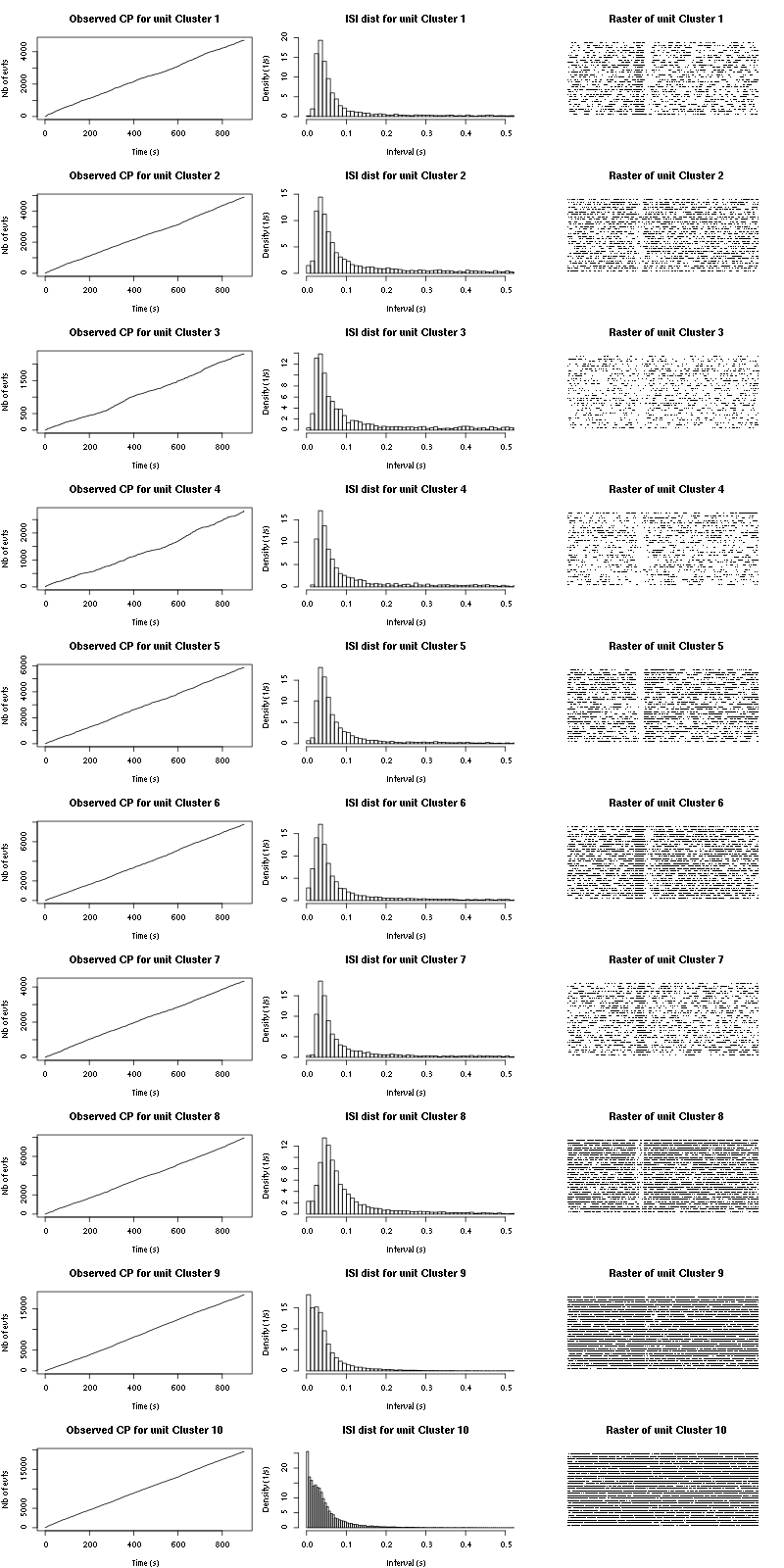
Figure 55: Observed counting processes, empirical inter spike interval distributions and raster plots for C3H_3.

The BRT and RFT tests give for the first 7 units:

layout_matrix = matrix(0,nr=nbc-3,nc=nbc-3)
counter = 1
for (i in 1:(nbc-3))
    for (j in 1:(nbc-3))
        if (i != j) {
            layout_matrix[i,j] = counter
            counter = counter +1
        }
layout(layout_matrix)
par(mar=c(4,3,4,1))
for (i in 1:(nbc-3))
    for (j in 1:(nbc-3))
        if (i != j)
            test_rt(a_C3H_3_tetB$spike_trains[[i]],
                    a_C3H_3_tetB$spike_trains[[j]],
		    nbins=200,single_trial_duration=30,
                    ylab="",main=paste("Units",i,"and",j))

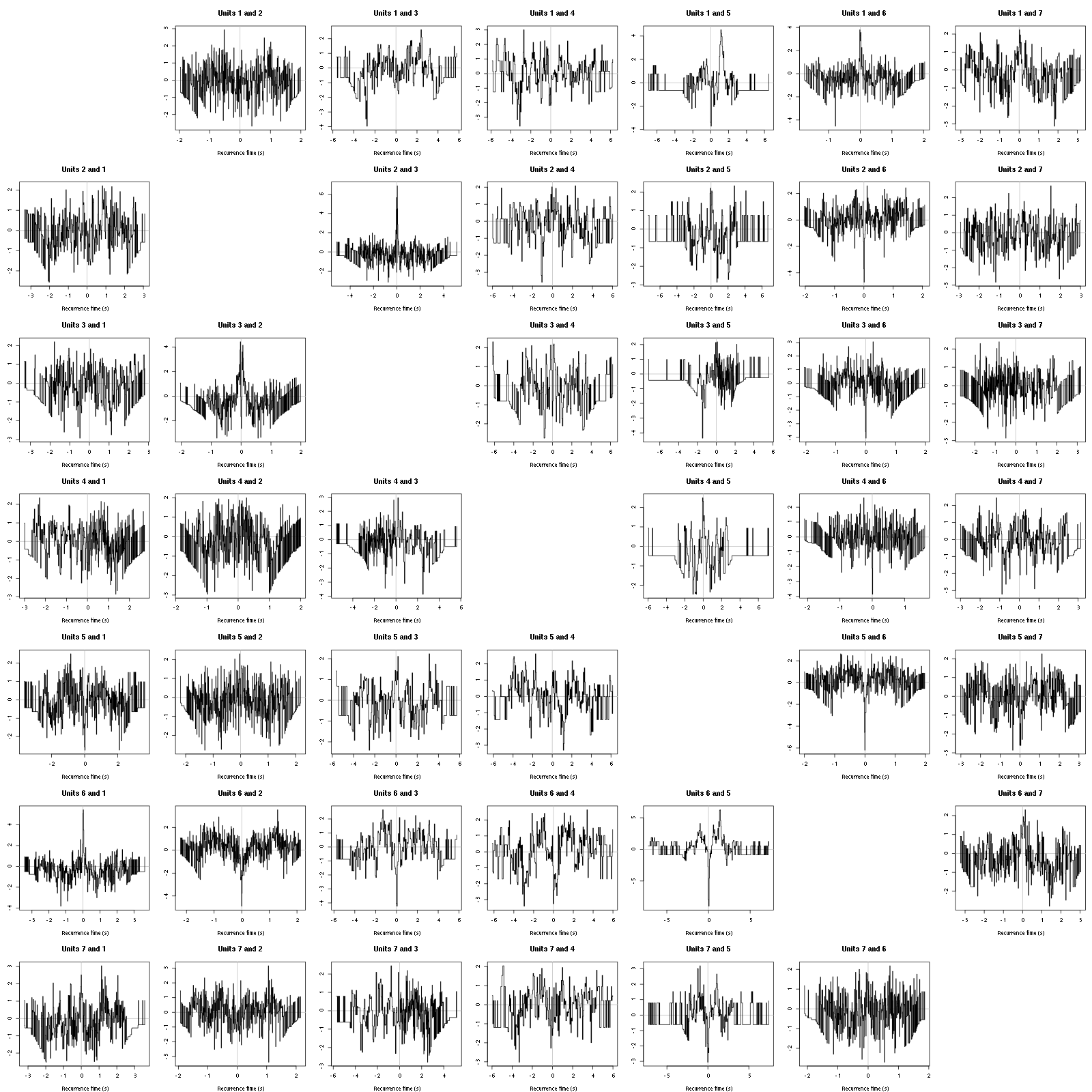
Figure 56: Graphical tests for the first 7 units of the Backward and Forward Reccurrence Times distribution against the null hypothesis (no interaction) during Spontaenous_1. If the null is correct, the curves should be IID draws from a standard normal distribution.

14.3 Save results

Before analyzing the next set of trials we save the output of sort_many_trials to disk with:

save(a_C3H_3_tetB,
     file=paste0("tetB_analysis/tetB_",stim_name,"_summary_obj.rda"))

We write to disk the spike trains in text mode:

for (c_idx in 1:length(a_C3H_3_tetB$spike_trains))
    if (!is.null(a_C3H_3_tetB$spike_trains[[c_idx]]))
        cat(a_C3H_3_tetB$spike_trains[[c_idx]],file=paste0("locust20010214_spike_trains/locust20010214_C3H_3_tetB_u",c_idx,".txt"),sep="\n")

15 10 trials of `C3H_4`

The LabBook mentions that the disk got filled up during trial 11 (30 were planed ) so we stop at trial 10.

15.1 Do the job

stim_name = "C3H_4"
a_C3H_4_tetB=sort_many_trials(inter_trial_time=30*15000,
                              get_data_fct=get_tetrode_data,
                              stim_name=stim_name,
                              trial_nbs=1:10,
                              centers=a_C3H_3_tetB$centers,
                              counts=a_C3H_3_tetB$counts,
                              all_at_once_call_list=list(thres=threshold_factor*c(1,1,1,1), 
                                                         filter_length_1=filter_length, filter_length=filter_length, 
                                                         minimalDist_1=15, minimalDist=15, 
                                                         before=c_before, after=c_after, 
                                                         detection_cycle=c(0,0), verbose=1),
                              layout_matrix=matrix(c(1,1:11),nr=6),new_weight_in_update=0.01
                              )

15.2 Diagnostic plots

The counts evolution is:

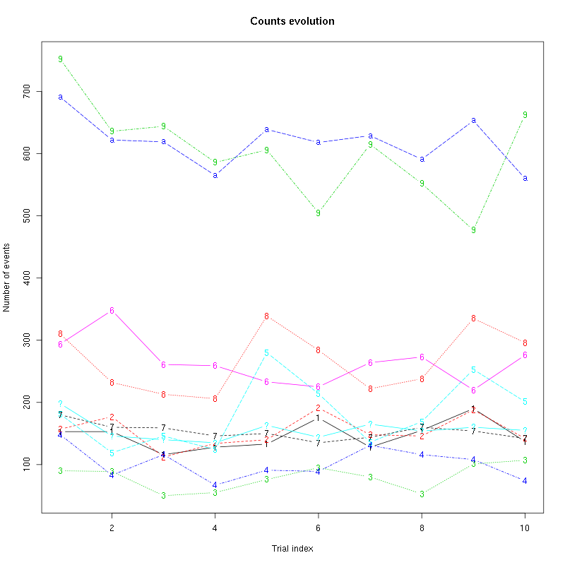
Figure 57: Evolution of the number of events attributed to each unit (1 to 9 and "a") or unclassified ("?") during the 10 trials of C3H_4 for tetrodeB.

The waveform evolution is:

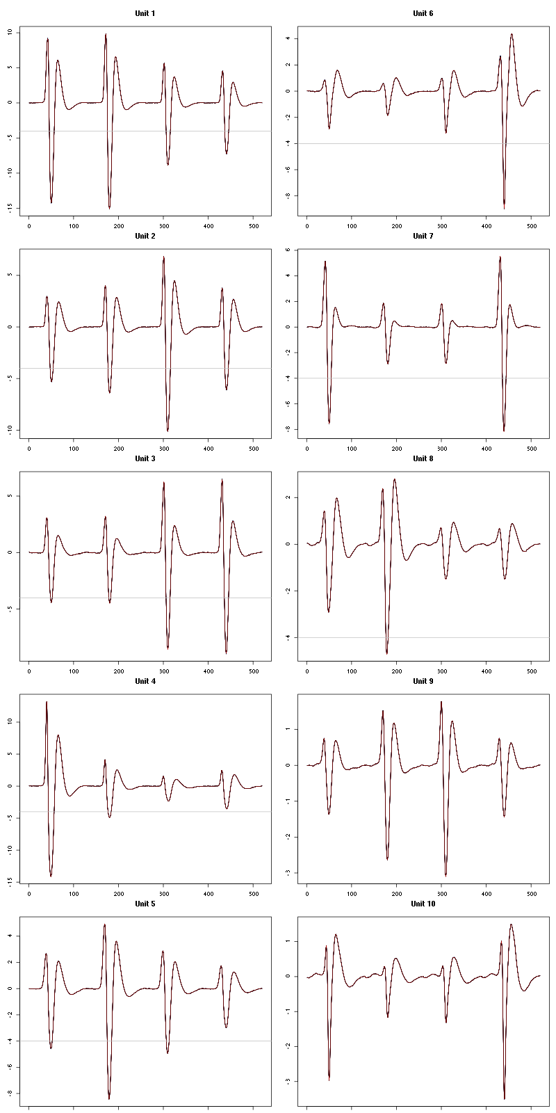
Figure 58: Evolution of the templates of each unit during the 10 trials of C3H_4 for tetrodeB.

The observed counting processes and inter spike intervals densities are:

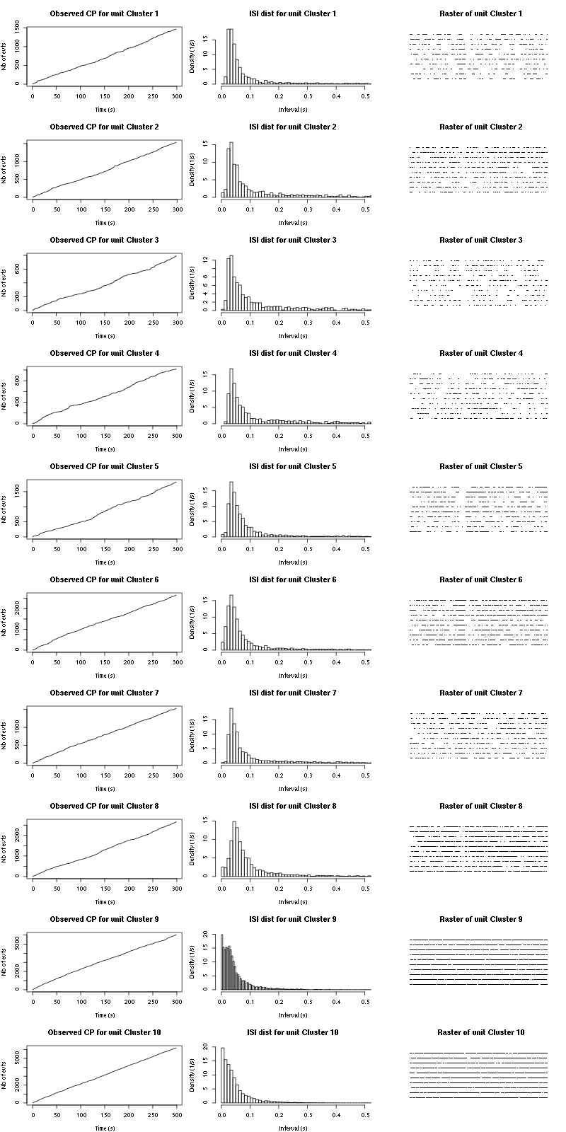
Figure 59: Observed counting processes, empirical inter spike interval distributions and raster plots for C3H_4.

The BRT and RFT tests give for the first 7 units:

layout_matrix = matrix(0,nr=nbc-3,nc=nbc-3)
counter = 1
for (i in 1:(nbc-3))
    for (j in 1:(nbc-3))
        if (i != j) {
            layout_matrix[i,j] = counter
            counter = counter +1
        }
layout(layout_matrix)
par(mar=c(4,3,4,1))
for (i in 1:(nbc-3))
    for (j in 1:(nbc-3))
        if (i != j)
            test_rt(a_C3H_4_tetB$spike_trains[[i]],
                    a_C3H_4_tetB$spike_trains[[j]],
		    nbins=200,single_trial_duration=30,
                    ylab="",main=paste("Units",i,"and",j))

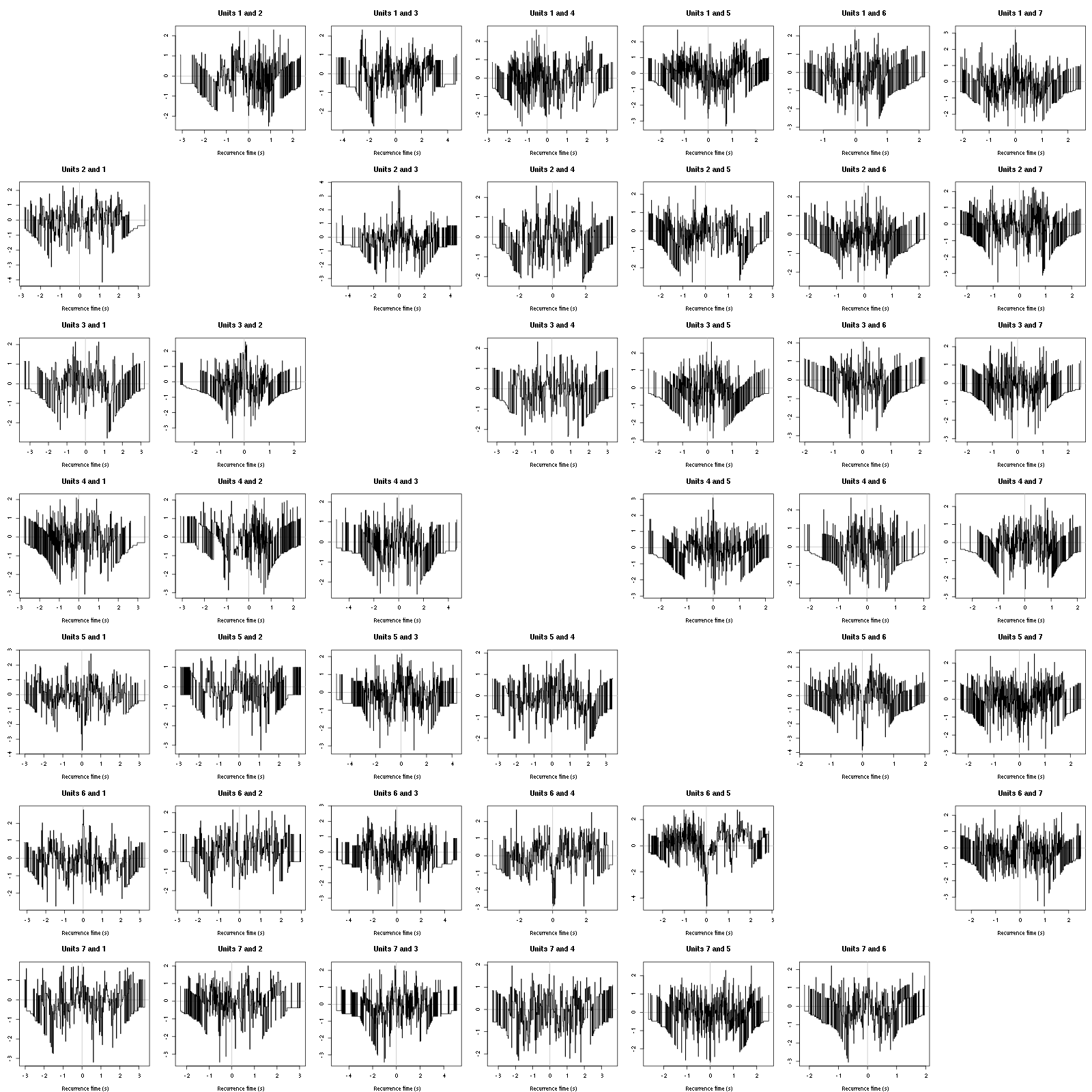
Figure 60: Graphical tests for the first 7 units of the Backward and Forward Reccurrence Times distribution against the null hypothesis (no interaction) during Spontaenous_1. If the null is correct, the curves should be IID draws from a standard normal distribution.

15.3 Save results

Before analyzing the next set of trials we save the output of sort_many_trials to disk with:

save(a_C3H_4_tetB,
     file=paste0("tetB_analysis/tetB_",stim_name,"_summary_obj.rda"))

We write to disk the spike trains in text mode:

for (c_idx in 1:length(a_C3H_4_tetB$spike_trains))
    if (!is.null(a_C3H_4_tetB$spike_trains[[c_idx]]))
        cat(a_C3H_4_tetB$spike_trains[[c_idx]],file=paste0("locust20010214_spike_trains/locust20010214_C3H_4_tetB_u",c_idx,".txt"),sep="\n")

16 30 trials of `C3H_5`

The LabBook mentions noise in trials 21, 22 and 23 so we do not consider them.

16.1 Do the job

stim_name = "C3H_5"
a_C3H_5_tetB=sort_many_trials(inter_trial_time=30*15000,
                              get_data_fct=get_tetrode_data,
                              stim_name=stim_name,
                              trial_nbs=c(1:20,24:30),
                              centers=a_C3H_4_tetB$centers,
                              counts=a_C3H_4_tetB$counts,
                              all_at_once_call_list=list(thres=threshold_factor*c(1,1,1,1), 
                                                         filter_length_1=filter_length, filter_length=filter_length, 
                                                         minimalDist_1=15, minimalDist=15, 
                                                         before=c_before, after=c_after, 
                                                         detection_cycle=c(0,0), verbose=1),
                              layout_matrix=matrix(c(1,1:11),nr=6),new_weight_in_update=0.01
                              )

16.2 Diagnostic plots

The counts evolution is:

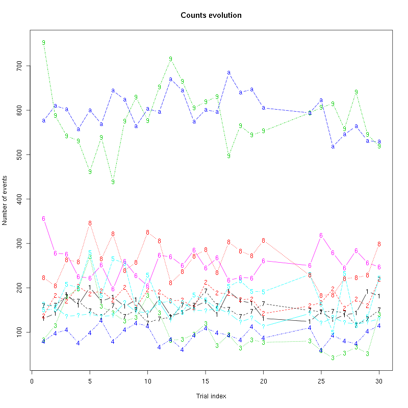
Figure 61: Evolution of the number of events attributed to each unit (1 to 9 and "a") or unclassified ("?") during the 27 trials of C3H_5 for tetrodeB.

The waveform evolution is:

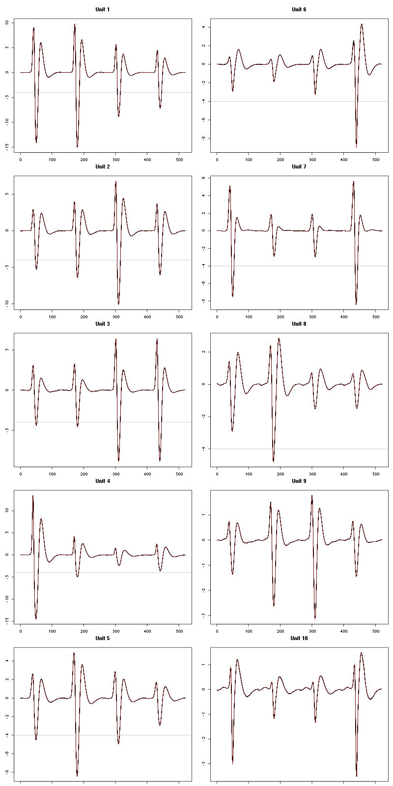
Figure 62: Evolution of the templates of each unit during the 27 trials of C3H_5 for tetrodeB.

The observed counting processes and inter spike intervals densities are:

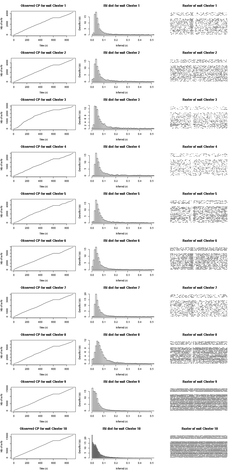
Figure 63: Observed counting processes, empirical inter spike interval distributions and raster plots for C3H_5.

The BRT and RFT tests give for the first 7 units:

layout_matrix = matrix(0,nr=nbc-3,nc=nbc-3)
counter = 1
for (i in 1:(nbc-3))
    for (j in 1:(nbc-3))
        if (i != j) {
            layout_matrix[i,j] = counter
            counter = counter +1
        }
layout(layout_matrix)
par(mar=c(4,3,4,1))
for (i in 1:(nbc-3))
    for (j in 1:(nbc-3))
        if (i != j)
            test_rt(a_C3H_5_tetB$spike_trains[[i]],
                    a_C3H_5_tetB$spike_trains[[j]],
		    nbins=200,single_trial_duration=30,
                    ylab="",main=paste("Units",i,"and",j))

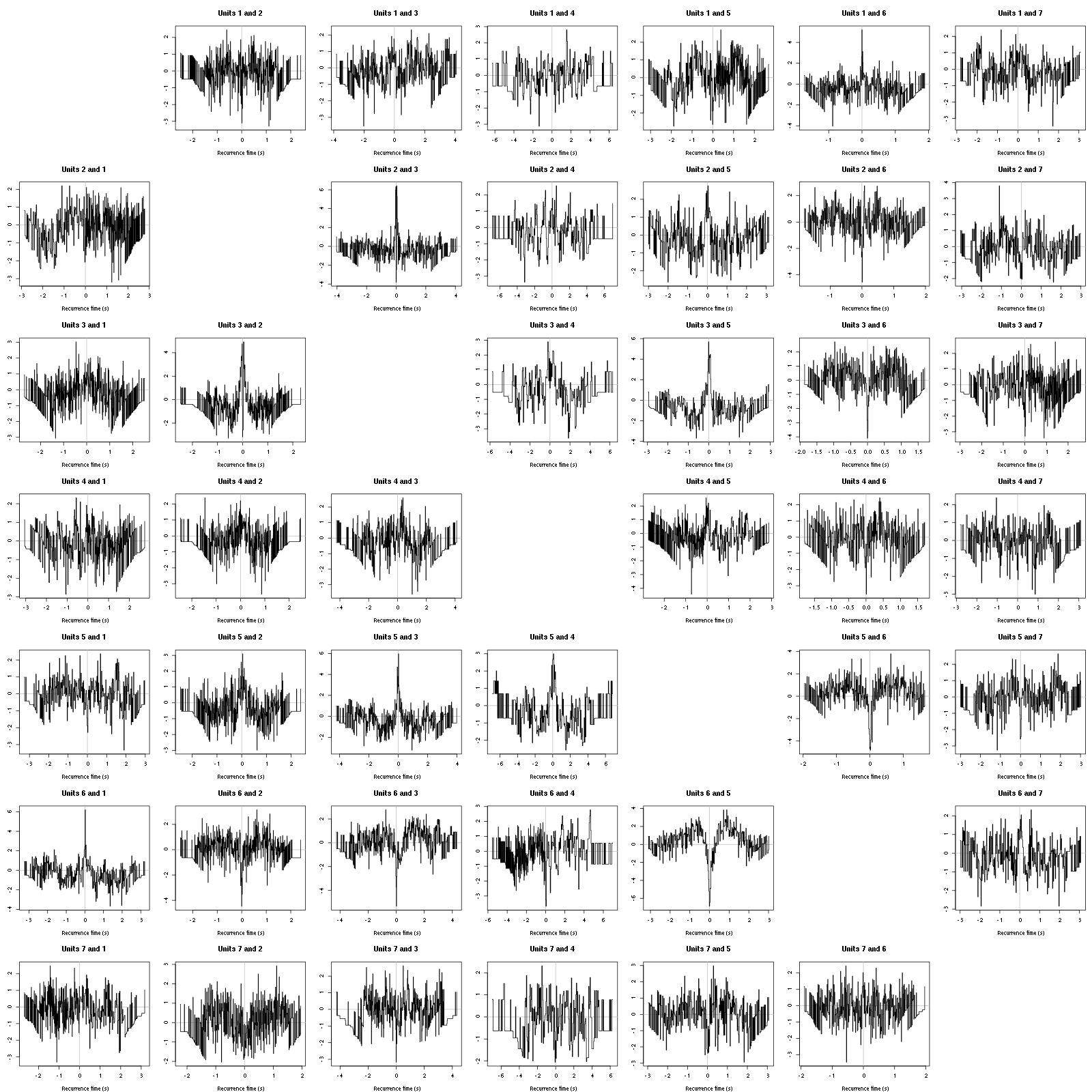
Figure 64: Graphical tests for the first 7 units of the Backward and Forward Reccurrence Times distribution against the null hypothesis (no interaction) during Spontaenous_1. If the null is correct, the curves should be IID draws from a standard normal distribution.

16.3 Save results

Before analyzing the next set of trials we save the output of sort_many_trials to disk with:

save(a_C3H_5_tetB,
     file=paste0("tetB_analysis/tetB_",stim_name,"_summary_obj.rda"))

We write to disk the spike trains in text mode:

for (c_idx in 1:length(a_C3H_5_tetB$spike_trains))
    if (!is.null(a_C3H_5_tetB$spike_trains[[c_idx]]))
        cat(a_C3H_5_tetB$spike_trains[[c_idx]],file=paste0("locust20010214_spike_trains/locust20010214_C3H_5_tetB_u",c_idx,".txt"),sep="\n")

17 30 trials of `C3H_6`

17.1 Do the job

stim_name = "C3H_6"
a_C3H_6_tetB=sort_many_trials(inter_trial_time=30*15000,
                              get_data_fct=get_tetrode_data,
                              stim_name=stim_name,
                              trial_nbs=1:30,
                              centers=a_C3H_5_tetB$centers,
                              counts=a_C3H_5_tetB$counts,
                              all_at_once_call_list=list(thres=threshold_factor*c(1,1,1,1), 
                                                         filter_length_1=filter_length, filter_length=filter_length, 
                                                         minimalDist_1=15, minimalDist=15, 
                                                         before=c_before, after=c_after, 
                                                         detection_cycle=c(0,0), verbose=1),
                              layout_matrix=matrix(c(1,1:11),nr=6),new_weight_in_update=0.01
                              )

17.2 Diagnostic plots

The counts evolution is:

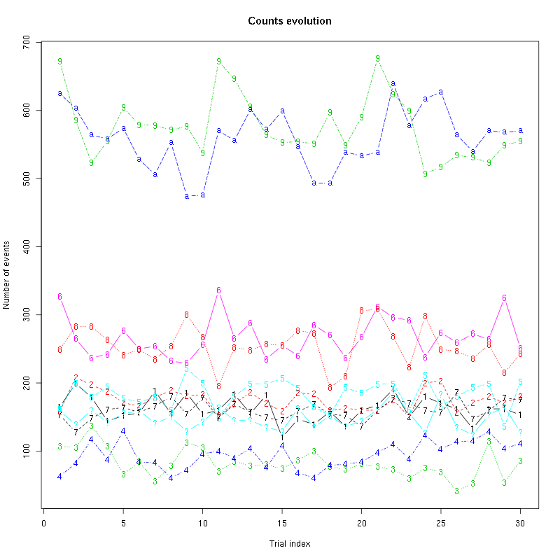
Figure 65: Evolution of the number of events attributed to each unit (1 to 9 and "a") or unclassified ("?") during the 30 trials of C3H_6 for tetrodeB.

The waveform evolution is:

Figure 66: Evolution of the templates of each unit during the 30 trials of C3H_6 for tetrodeB.

The observed counting processes and inter spike intervals densities are:

Figure 67: Observed counting processes, empirical inter spike interval distributions and raster plots for C3H_6.

The BRT and RFT tests give for the first 7 units:

layout_matrix = matrix(0,nr=nbc-3,nc=nbc-3)
counter = 1
for (i in 1:(nbc-3))
    for (j in 1:(nbc-3))
        if (i != j) {
            layout_matrix[i,j] = counter
            counter = counter +1
        }
layout(layout_matrix)
par(mar=c(4,3,4,1))
for (i in 1:(nbc-3))
    for (j in 1:(nbc-3))
        if (i != j)
            test_rt(a_C3H_6_tetB$spike_trains[[i]],
                    a_C3H_6_tetB$spike_trains[[j]],
		    nbins=200,single_trial_duration=30,
                    ylab="",main=paste("Units",i,"and",j))

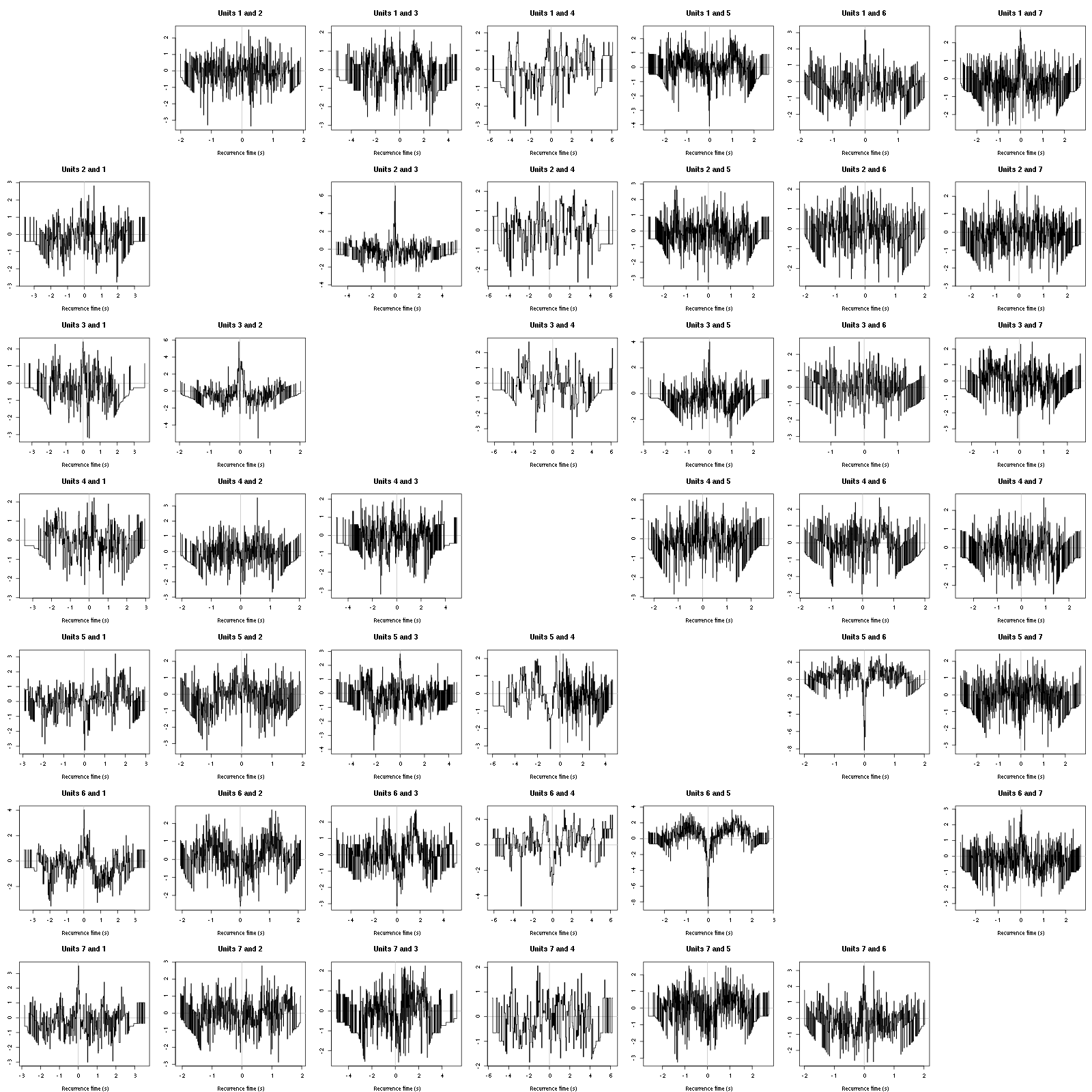
Figure 68: Graphical tests for the first 7 units of the Backward and Forward Reccurrence Times distribution against the null hypothesis (no interaction) during Spontaenous_1. If the null is correct, the curves should be IID draws from a standard normal distribution.

17.3 Save results

Before analyzing the next set of trials we save the output of sort_many_trials to disk with:

save(a_C3H_6_tetB,
     file=paste0("tetB_analysis/tetB_",stim_name,"_summary_obj.rda"))

We write to disk the spike trains in text mode:

for (c_idx in 1:length(a_C3H_6_tetB$spike_trains))
    if (!is.null(a_C3H_6_tetB$spike_trains[[c_idx]]))
        cat(a_C3H_6_tetB$spike_trains[[c_idx]],file=paste0("locust20010214_spike_trains/locust20010214_C3H_6_tetB_u",c_idx,".txt"),sep="\n")

Sorting data set 20010214 tetrode B (channels 2, 3, 5, 7)

Table of Contents

1 Introduction

1.1 Getting the data

1.2 Getting the code

2 Tetrode B (channels 2, 3, 5, 7) analysis

2.1 Loading the data

2.2 Five number summary

2.3 Plot the data

2.4 Data normalization

2.5 Spike detection

2.6 Cuts

2.7 Events

2.8 Removing obvious superposition

2.9 Dimension reduction

2.10 Exporting for GGobi

2.11 kmeans clustering with 10

2.12 Long cuts creation

2.13 Peeling

2.13.1 Round 0

2.13.2 Round 1

2.14 Getting the spike trains

2.15 Getting the inter spike intervals and the forward and backward recurrence times

2.15.1 ISI distributions

2.15.2 Forward and Backward Recurrence Times

2.16 Making "all at once"

2.16.1 What should our "all at once" function do?

2.16.2 all_at_once definition

2.16.3 Test

3 Analyzing a sequence of trials

3.1 Create a directory were results get saved

3.2 Create a data loading function

3.3 sort_many_trials definition

3.4 Diagnostic plot function definitions

4 Systematic analysis of the 30 trials from Spontaneous_2 backwards

4.1 Doing the job

4.2 Diagnostic plots

4.3 Save results

5 30 trials of Spontaenous_1 backwards

5.1 Do the job

5.2 Diagnostic plots

5.3 Save results

6 25 trials with Cis-3-Hexen-1-ol (C3H_1)

6.1 Do the job

6.2 Diagnostic plots

6.3 Save results

7 25 trials with Citral

7.1 Do the job

7.2 Diagnostic plots

7.3 Save results

8 25 trials with Vanilla

8.1 Do the job

8.2 Diagnostic plots

8.3 Save results

9 25 trials with Octanol

9.1 Do the job

9.2 Diagnostic plots

9.3 Save results

10 25 trials with Mint

10.1 Do the job

10.2 Diagnostic plots

10.3 Save results

11 25 trials with C3H_2

11.1 Do the job

11.2 Diagnostic plots

11.3 Save results

12 30 trials of Spontaneous_3

12.1 Redefine get_tetrode_data

12.2 Do the job

12.3 Diagnostic plots

12.4 Save results

13 30 trials of Spontaneous_4

13.1 Do the job

13.2 Diagnostic plots

13.3 Save results

14 30 trials of C3H_3

14.1 Do the job

14.2 Diagnostic plots

14.3 Save results

15 10 trials of C3H_4

2.10 Exporting for `GGobi`

2.16.2 `all_at_once` definition

3.3 `sort_many_trials` definition

4 Systematic analysis of the 30 trials from `Spontaneous_2` backwards

5 30 trials of `Spontaenous_1` backwards

6 25 trials with `Cis-3-Hexen-1-ol` (`C3H_1`)

7 25 trials with `Citral`

8 25 trials with `Vanilla`

9 25 trials with `Octanol`

10 25 trials with `Mint`

11 25 trials with `C3H_2`

12 30 trials of `Spontaneous_3`

12.1 Redefine `get_tetrode_data`

13 30 trials of `Spontaneous_4`

14 30 trials of `C3H_3`

15 10 trials of `C3H_4`

16 30 trials of `C3H_5`

17 30 trials of `C3H_6`