Sorting data set 20010217 tetrode D (channels 10, 12, 14, 15)

1. Introduction
- 1.1. Getting the data
- 1.2. Getting the code
2. Tetrode B (channels 10, 12, 14, 15) analysis

1 Introduction

This is the description of how to do the (spike) sorting of tetrode D (channels 10, 12, 14, 15) from data set locust20010217.

1.1 Getting the data

The data are split into two HDF5 files, locust20010217_part1.hdf5 and locust20010217_part2.hdf5, located on zenodo and can be downloaded interactivelly with a web browser or by typing at the command line:

wget https://zenodo.org/record/21589/files/locust20010217.hdf5

In the sequel I will assume that R has been started in the directory where the data were downloaded (in other words, the working direcory should be the one containing the data.

The data are in HDF5 format and the easiest way to get them into R is to install the rhdf5 package from Bioconductor. Once the installation is done, the library is loaded into R with:

library(rhdf5)

We can then get a (long and detailed) listing of our data file content with (result not shown):

h5ls("locust20010217_part1.hdf5")

There must be functions to get access to the metadata contained in the file with rhdf5 but I do not know them so I'm using HDFView called from the command line for that. All the relevant information about the experiment are stored in these metadata so you should take a look at them.

1.2 Getting the code

The code can be sourced as follows:

source("https://raw.githubusercontent.com/christophe-pouzat/zenodo-locust-datasets-analysis/master/R_Sorting_Code/sorting_with_r.R")

A description of the functions contained in this file can be found at the following address: http://xtof.perso.math.cnrs.fr/locust.html.

2 Tetrode B (channels 10, 12, 14, 15) analysis

We now want to get our "model", that is a dictionnary of waveforms (one waveform per neuron and per recording site). To that end we are going to use the first 29 s of data contained in the Spontaneous_1/trial_01 Group (in HDF5 jargon).

2.1 Loading the data

So we start by loading the data from channels 10, 12, 14, 15 into R:

lD = get_data(1,"Spontaneous 1",
              channels = c("ch10","ch12","ch14","ch15"),
              file="locust20010217.hdf5")
dim(lD)

431548

2.2 Five number summary

We get the Five number summary with:

summary(lD,digits=2)

Min. :1626	Min. :1486	Min. :1432	Min. :1665
1st Qu.:2014	1st Qu.:2005	1st Qu.:2001	1st Qu.:2010
Median :2045	Median :2045	Median :2044	Median :2046
Mean :2045	Mean :2045	Mean :2044	Mean :2046
3rd Qu.:2077	3rd Qu.:2086	3rd Qu.:2088	3rd Qu.:2082
Max. :2383	Max. :2495	Max. :2526	Max. :2378

It shows that the channels have very similar properties as far as the median and the inter-quartile range (IQR) are concerned. The minimum is much smaller on the third channel. This suggests that the largest spikes are going to be found here (remember that spikes are going mainly downwards).

2.3 Plot the data

We "convert" the data matrix lD into a time series object with:

lD = ts(lD,start=0,freq=15e3)

We can then plot the whole data with (not shown since it makes a very figure):

plot(lD)

2.4 Data normalization

As always we normalize such that the median absolute deviation (MAD) becomes 1:

lD.mad = apply(lD,2,mad)
lD = t((t(lD)-apply(lD,2,median))/lD.mad)
lD = ts(lD,start=0,freq=15e3)

Once this is done we explore interactively the data with:

explore(lD,col=c("black","grey70"))

Most spikes can be seen on the 4 recording sites and there are different spike waveform!

2.5 Spike detection

Since the spikes are mainly going downwards, we will detect valleys instead of peaks:

lDf = -lD
filter_length = 5
threshold_factor = 4
lDf = filter(lDf,rep(1,filter_length)/filter_length)
lDf[is.na(lDf)] = 0
lDf.mad = apply(lDf,2,mad)
lDf_mad_original = lDf.mad
lDf = t(t(lDf)/lDf_mad_original)
thrs = threshold_factor*c(1,1,1,1)
bellow.thrs = t(t(lDf) < thrs)
lDfr = lDf
lDfr[bellow.thrs] = 0
remove(lDf)
sp0 = peaks(apply(lDfr,1,sum),15)
remove(lDfr)
sp0

eventsPos object with indexes of 1307 events. 
  Mean inter event interval: 329.95 sampling points, corresponding SD: 329.71 sampling points 
  Smallest and largest inter event intervals: 16 and 2961 sampling points.

Every time a filter length / threshold combination is tried, the detection is checked interactively with:

explore(sp0,lD,col=c("black","grey50"))

2.6 Cuts

We proceed as usual to get the cut length right:

evts = mkEvents(sp0,lD,49,50)
evts.med = median(evts)
evts.mad = apply(evts,1,mad)
plot_range = range(c(evts.med,evts.mad))
plot(evts.med,type="n",ylab="Amplitude",
     ylim=plot_range)
abline(v=seq(0,400,10),col="grey")
abline(h=c(0,1),col="grey")
lines(evts.med,lwd=2)
lines(evts.mad,col=2,lwd=2)

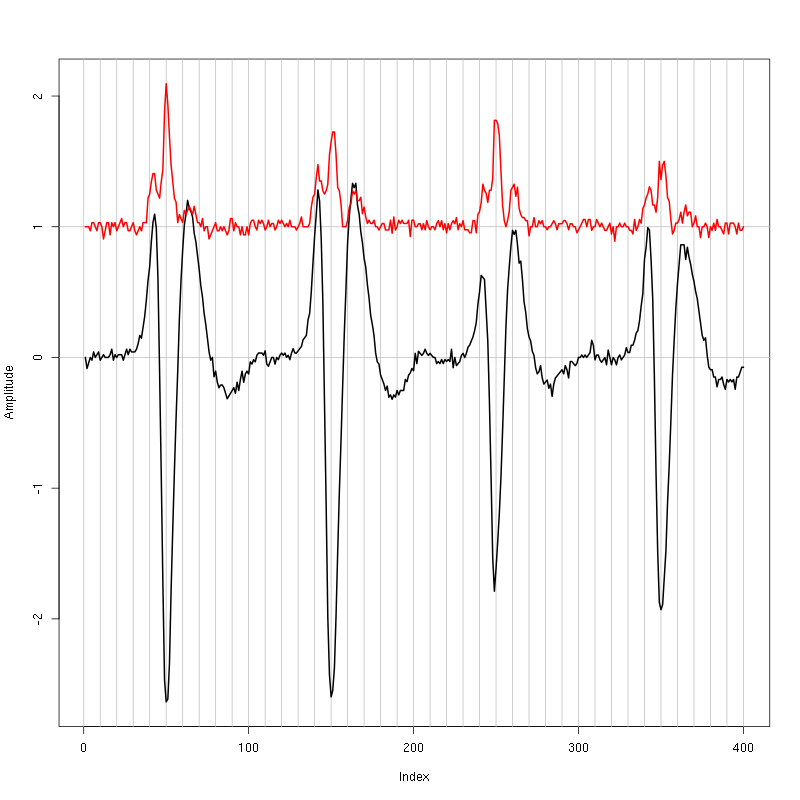
Figure 1: Setting the cut length for the data from tetrode D (channels 10, 12, 14, 15). We see that we need 15 points before the peak and 30 after.

We see that we need roughly 15 points before the peak and 30 after.

2.7 Events

We now cut our events:

evts = mkEvents(sp0,lD,14,30)
summary(evts)

events object deriving from data set: lD.
 Events defined as cuts of 45 sampling points on each of the 4 recording sites.
 The 'reference' time of each event is located at point 15 of the cut.
 There are 1307 events in the object.

We can as usual visualize the first 200 events with:

evts[,1:200]

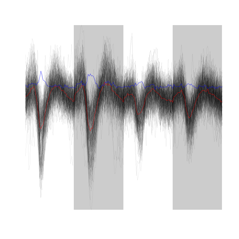
Figure 2: First 200 events for the data from tetrode D (channels 1, 3, 5, 7).

We do see some superposition and it's therefore a good idea to remove the most obvious of them before reducing the dimension.

2.8 Removing obvious superposition

We define function goodEvtsFct with:

goodEvtsFct = function(samp,thr=3) {
    samp.med = apply(samp,1,median)
    samp.mad = apply(samp,1,mad)
    below = samp.med < 0
    samp.r = apply(samp,2,function(x) {x[below] = 0;x})
    apply(samp.r,2,function(x) all(abs(x-samp.med) < thr*samp.mad))
}

We apply it with a threshold of 5 times the MAD:

goodEvts = goodEvtsFct(evts,5)

2.9 Dimension reduction

We do a PCA on our good events set:

evts.pc = prcomp(t(evts[,goodEvts]))

We look at the projections on the first 4 principle components:

panel.dens = function(x,...) {
  usr = par("usr")
  on.exit(par(usr))
  par(usr = c(usr[1:2], 0, 1.5) )
  d = density(x, adjust=0.5)
  x = d$x
  y = d$y
  y = y/max(y)
  lines(x, y, col="grey50", ...)
}
pairs(evts.pc$x[,1:4],pch=".",gap=0,diag.panel=panel.dens)

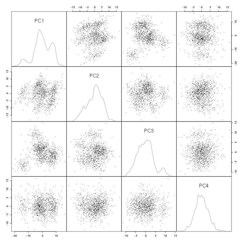
Figure 3: The good events from tetrode D (channels 10, 12, 14, 15) projected onto the first 4 PCs.

I see 6/7 clusters. We can also look at the projections on the PC pairs defined by the next 4 PCs:

pairs(evts.pc$x[,5:8],pch=".",gap=0,diag.panel=panel.dens)

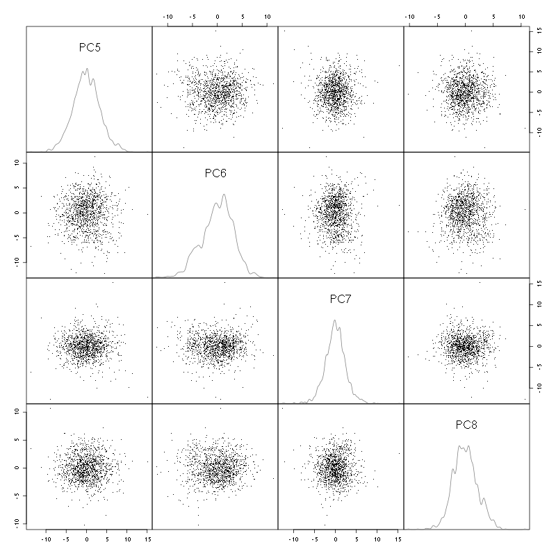
Figure 4: The good events from tetrode D (channels 10, 12, 14, 15) projected onto PC 5 to 8.

There is not much structure left beyond the 4th PC.

2.10 Exporting for `GGobi`

We export the events projected onto the first 8 principle components in csv format:

write.csv(evts.pc$x[,1:8],file="tetD_evts.csv")

Using the rotation display of GGobi with the first 3 principle components and the 2D tour with the first 4 components I see 8 clusters. So we will start with a kmeans with 8 centers.

2.11 kmeans clustering with 8 clusters

nbc=8
set.seed(20110928,kind="Mersenne-Twister")
km = kmeans(evts.pc$x[,1:4],centers=nbc,iter.max=100,nstart=100)
label = km$cluster
cluster.med = sapply(1:nbc, function(cIdx) median(evts[,goodEvts][,label==cIdx]))
sizeC = sapply(1:nbc,function(cIdx) sum(abs(cluster.med[,cIdx])))
newOrder = sort.int(sizeC,decreasing=TRUE,index.return=TRUE)$ix
cluster.mad = sapply(1:nbc, function(cIdx) {ce = t(evts[,goodEvts]);ce = ce[label==cIdx,];apply(ce,2,mad)})
cluster.med = cluster.med[,newOrder]
cluster.mad = cluster.mad[,newOrder]
labelb = sapply(1:nbc, function(idx) (1:nbc)[newOrder==idx])[label]

We write a new csv file with the data and the labels:

write.csv(cbind(evts.pc$x[,1:4],labelb),file="tetD_sorted.csv")

That looks good!

We get a plot showing the events attributed to each of the first 4 units with:

layout(matrix(1:4,nr=4))
par(mar=c(1,1,1,1))
for (i in (1:4)) plot(evts[,goodEvts][,labelb==i],y.bar=5)

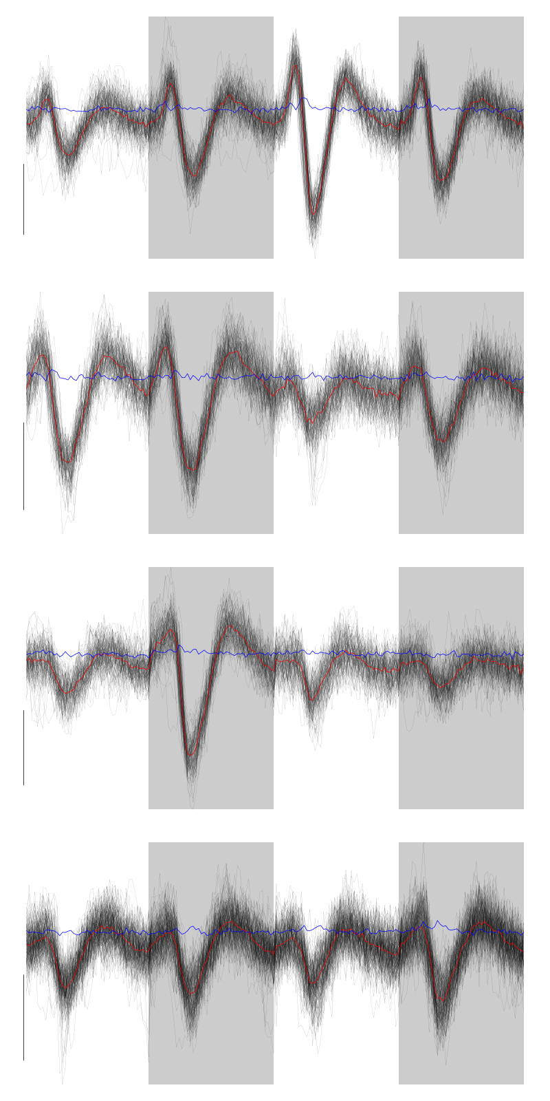
Figure 5: The events of the first four clusters of tetrode D

We get a plot showing the events attributed to each of the last 4 units with:

layout(matrix(1:4,nr=4))
par(mar=c(1,1,1,1))
for (i in (5:8)) plot(evts[,goodEvts][,labelb==i],y.bar=5)

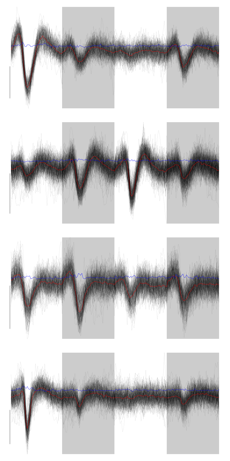
Figure 6: The events of the last four clusters of tetrode D

In fact I see rather 2 units in cluster 4 and 7 so I redo the clustering with 10 units

2.12 kmeans clustering with 10 clusters

nbc=10
set.seed(20110928,kind="Mersenne-Twister")
km = kmeans(evts.pc$x[,1:4],centers=nbc,iter.max=100,nstart=100)
label = km$cluster
cluster.med = sapply(1:nbc, function(cIdx) median(evts[,goodEvts][,label==cIdx]))
sizeC = sapply(1:nbc,function(cIdx) sum(abs(cluster.med[,cIdx])))
newOrder = sort.int(sizeC,decreasing=TRUE,index.return=TRUE)$ix
cluster.mad = sapply(1:nbc, function(cIdx) {ce = t(evts[,goodEvts]);ce = ce[label==cIdx,];apply(ce,2,mad)})
cluster.med = cluster.med[,newOrder]
cluster.mad = cluster.mad[,newOrder]
labelb = sapply(1:nbc, function(idx) (1:nbc)[newOrder==idx])[label]

We get a plot showing the events attributed to each of the first 5 units with:

layout(matrix(1:5,nr=5))
par(mar=c(1,1,1,1))
for (i in (1:5)) plot(evts[,goodEvts][,labelb==i],y.bar=5)

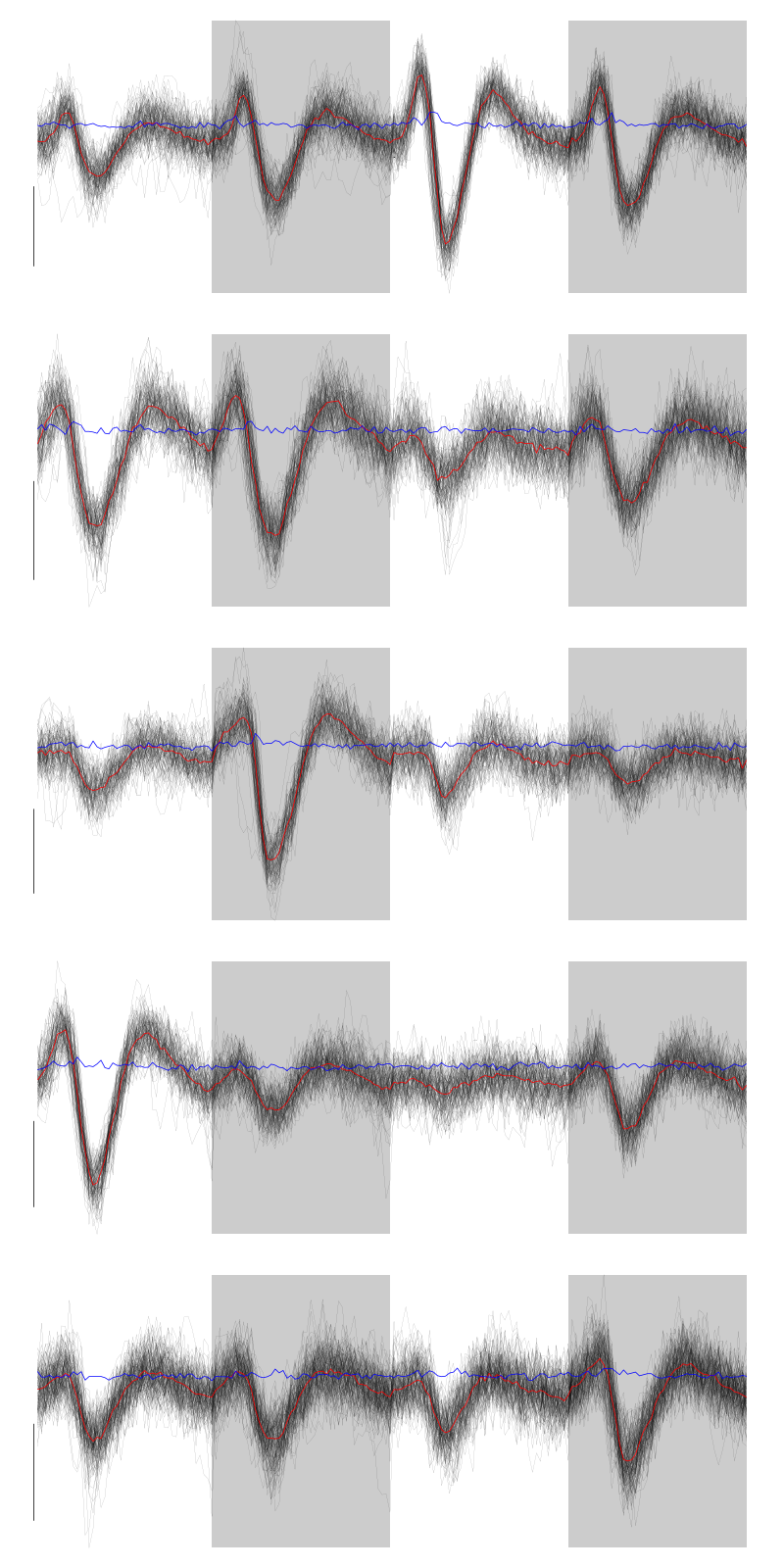
Figure 7: The events of the first five clusters of tetrode D

We get a plot showing the events attributed to each of the last 5 units with:

layout(matrix(1:5,nr=5))
par(mar=c(1,1,1,1))
for (i in (6:10)) plot(evts[,goodEvts][,labelb==i],y.bar=5)

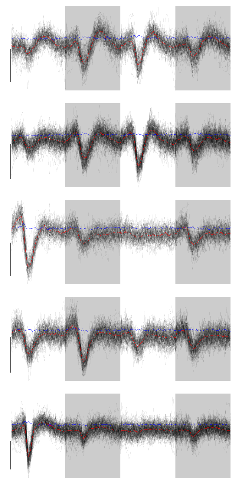
Figure 8: The events of the last five clusters of tetrode D

2.13 Long cuts creation

For the peeling process we need templates that start and end at 0 (we will otherwise generate artifacts when we subtract). We proceed "as usual" with (I tried first with the default value for parameters before and after but I reduced their values after looking at the centers, see the next figure):

c_before = 49
c_after = 80
centers = lapply(1:nbc, function(i)
    mk_center_list(sp0[goodEvts][labelb==i],lD,
                   before=c_before,after=c_after))
names(centers) = paste("Cluster",1:nbc)

We then make sure that our cuts are long enough by looking at them. Starting with the first five clusters:

layout(matrix(1:5,nr=5))
par(mar=c(1,4,1,1))
the_range=c(min(sapply(centers,function(l) min(l$center))),
            max(sapply(centers,function(l) max(l$center))))
for (i in 1:5) {
    template = centers[[i]]$center
    plot(template,lwd=2,col=2,
         ylim=the_range,type="l",ylab="")
    abline(h=0,col="grey50")
    abline(v=(1:2)*(c_before+c_after)+1,col="grey50")
    lines(filter(template,rep(1,filter_length)/filter_length),
          col=1,lty=3,lwd=2)
    abline(h=-threshold_factor,col="grey",lty=2,lwd=2)
    lines(centers[[i]]$centerD,lwd=2,col=4)
}

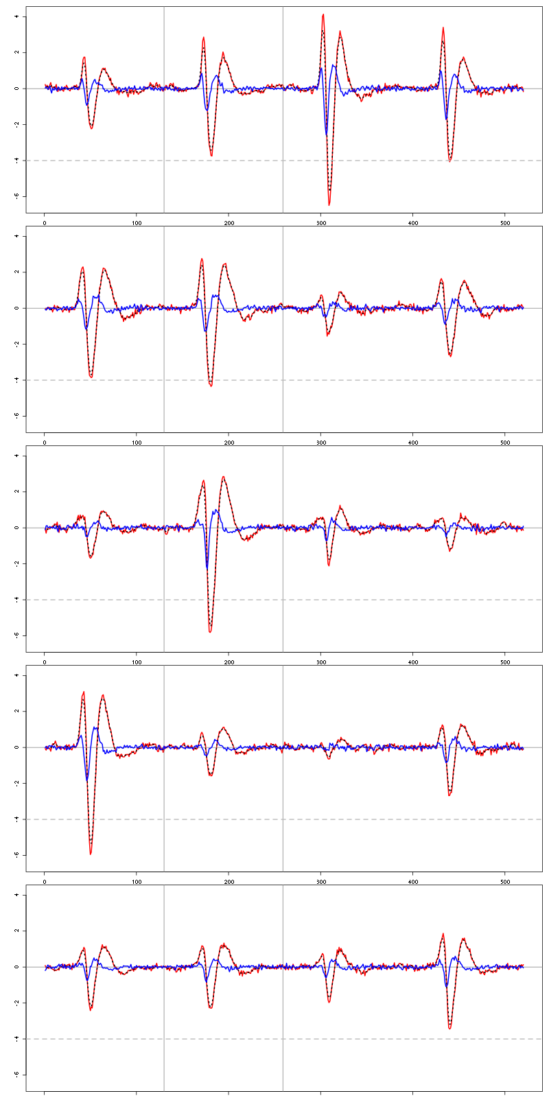
Figure 9: The first five templates (red) together with their first derivative (blue) all with the same scale.

The last five clusters:

layout(matrix(1:5,nr=5))
par(mar=c(1,4,1,1))
the_range=c(min(sapply(centers,function(l) min(l$center))),
            max(sapply(centers,function(l) max(l$center))))
for (i in 6:10) {
    template = centers[[i]]$center
    plot(template,lwd=2,col=2,
         ylim=the_range,type="l",ylab="")
    abline(h=0,col="grey50")
    abline(v=(1:2)*(c_before+c_after)+1,col="grey50")
    lines(filter(template,rep(1,filter_length)/filter_length),
          col=1,lty=3,lwd=2)
    abline(h=-threshold_factor,col="grey",lty=2,lwd=2)
    lines(centers[[i]]$centerD,lwd=2,col=4)
}

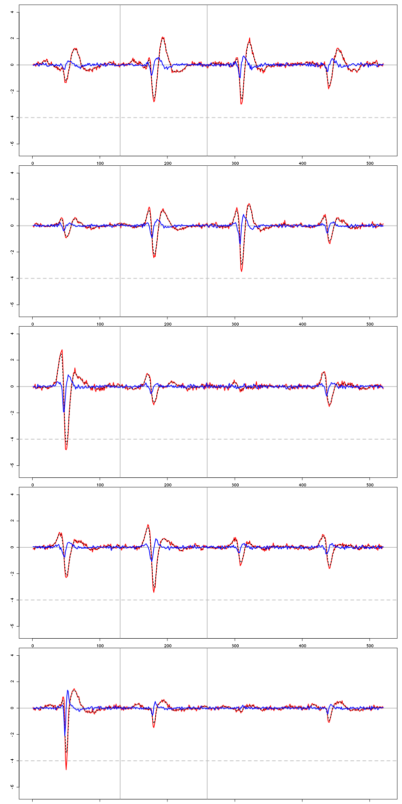
Figure 10: The last five templates (red) together with their first derivative (blue) all with the same scale.

We see that with our setting only units 1, 2, 3, 4 and 8 are going to be reliably detected.

2.14 Peeling

We can now do the peeling.

2.14.1 Round 0

We classify, predict, subtract and check how many non-classified events we get:

round0 = lapply(as.vector(sp0),classify_and_align_evt,
                data=lD,centers=centers,
                before=c_before,after=c_after)
pred0 = predict_data(round0,centers,data_length = dim(lD)[1])
lD_1 = lD - pred0
sum(sapply(round0, function(l) l[[1]] == '?'))

We can see the difference before / after peeling for the data between 1.0 and 1.1 s:

ii = 1:1500 + 1.0*15000
tt = ii/15000
par(mar=c(1,1,1,1))
plot(tt, lD[ii,1], axes = FALSE,
     type="l",ylim=c(-50,10),
     xlab="",ylab="")
lines(tt, lD_1[ii,1], col='red')
lines(tt, lD[ii,2]-15, col='black')
lines(tt, lD_1[ii,2]-15, col='red')
lines(tt, lD[ii,3]-25, col='black')
lines(tt, lD_1[ii,3]-25, col='red')
lines(tt, lD[ii,4]-40, col='black')
lines(tt, lD_1[ii,4]-40, col='red')

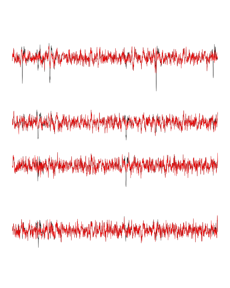
Figure 11: The first peeling illustrated on 100 ms of data, the raw data are in black and the first subtration in red.

2.14.2 Round 1

We keep going, using the subtracted data lD_1 as "raw data", detecting only all sites:

lDf = -lD_1
lDf = filter(lDf,rep(1,filter_length)/filter_length)
lDf[is.na(lDf)] = 0
lDf = t(t(lDf)/lDf_mad_original)
thrs = threshold_factor*c(1,1,1,1)
bellow.thrs = t(t(lDf) < thrs)
lDfr = lDf
lDfr[bellow.thrs] = 0
remove(lDf)
sp1 = peaks(apply(lDfr,1,sum),15)
remove(lDfr)
sp1

eventsPos object with indexes of 67 events. 
  Mean inter event interval: 6271.83 sampling points, corresponding SD: 7284.81 sampling points 
  Smallest and largest inter event intervals: 50 and 27732 sampling points.

We classify, predict, subtract and check how many non-classified events we get:

round1 = lapply(as.vector(sp1),classify_and_align_evt,
                data=lD_1,centers=centers,
                before=c_before,after=c_after)
pred1 = predict_data(round1,centers,data_length = dim(lD)[1])
lD_2 = lD_1 - pred1
sum(sapply(round1, function(l) l[[1]] == '?'))

We look at what's left with (not shown):

explore(sp1,lD_2,col=c("black","grey50"))

We decide to stop here.

2.15 Getting the spike trains

round_all = c(round0,round1)
spike_trains = lapply(paste("Cluster",1:nbc),
                      function(cn) sapply(round_all[sapply(round_all,
                                                           function(l) l[[1]]==cn)],
                                          function(l) l[[2]]+l[[3]]))
names(spike_trains) = paste("Cluster",1:nbc)

2.16 Getting the inter spike intervals and the forward and backward recurrence times

2.16.1 ISI distributions

We first get the ISI (inter spike intervals) of each unit:

isi = sapply(spike_trains, diff)
names(isi) = names(spike_trains)

We get the ISI ECDF for the units with:

layout(matrix(1:(nbc+nbc %% 2),nr=ceiling(nbc/2)))
par(mar=c(4,5,6,1))
for (cn in names(isi)) plot_isi(isi[[cn]],main=cn)

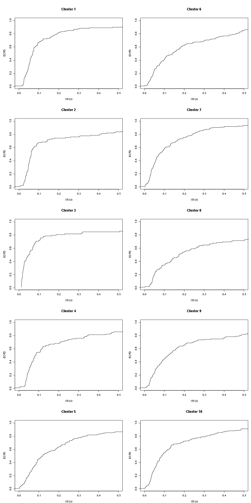
Figure 12: ISI ECDF for the ten units.

2.16.2 Forward and Backward Recurrence Times

On the data at hand that gives for units 1 to 7:

layout_matrix = matrix(0,nr=nbc-3,nc=nbc-3)
counter = 1
for (i in 1:(nbc-3))
    for (j in 1:(nbc-3))
        if (i != j) {
            layout_matrix[i,j] = counter
            counter = counter +1
        }
layout(layout_matrix)
par(mar=c(4,3,4,1))
for (i in 1:(nbc-3))
    for (j in 1:(nbc-3))
        if (i != j)
            test_rt(spike_trains[[i]],
                    spike_trains[[j]],
                    ylab="",main=paste("Units",i,"and",j))

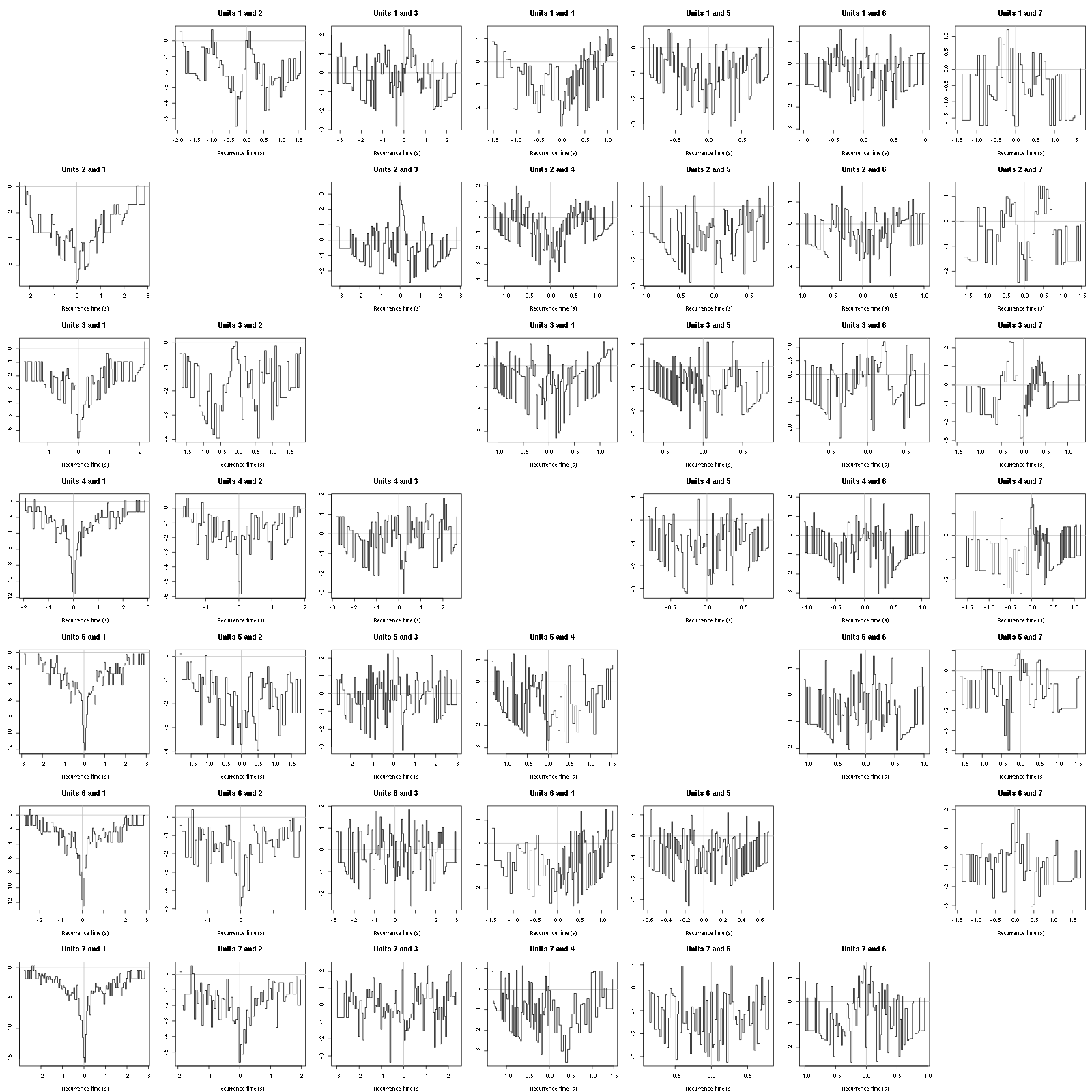
Figure 13: Graphical tests for the first 7 units of the Backward and Forward Reccurrence Times distrution agaisnt the null hypothesis (no interaction). If the null is correct, the curves should be IID draws from a standard normal distribution.

On this time scale with this number of events, there are a lot of signs of interactions.

2.17 `all_at_once` test

We test the function with:

## We need again an un-normalized version of the data
ref_data = get_data(1,"Spontaneous 1",
                    channels = c("ch10","ch12","ch14","ch15"),
                    file="locust20010217.hdf5")
## We can now use our function
aao=all_at_once(ref_data,centers,
                thres=threshold_factor*c(1,1,1,1),
                filter_length_1=filter_length,
                filter_length=filter_length,
                minimalDist_1=15,
                minimalDist=15,
                before=c_before,
                after=c_after,
                detection_cycle=c(0,0),
                verbose=2)

The five number summary is:
      ch10           ch12           ch14           ch15     
 Min.   :1626   Min.   :1486   Min.   :1432   Min.   :1665  
 1st Qu.:2014   1st Qu.:2005   1st Qu.:2001   1st Qu.:2010  
 Median :2045   Median :2045   Median :2044   Median :2046  
 Mean   :2045   Mean   :2045   Mean   :2044   Mean   :2046  
 3rd Qu.:2077   3rd Qu.:2086   3rd Qu.:2088   3rd Qu.:2082  
 Max.   :2383   Max.   :2495   Max.   :2526   Max.   :2378  

Doing now round 0 detecting on all sites
     Total  Cluster 1  Cluster 2  Cluster 3  Cluster 4  Cluster 5  Cluster 6 
      1307        119        115         99        112        144        123 
 Cluster 7  Cluster 8  Cluster 9 Cluster 10          ? 
       180         99        134        180          2 

Doing now round 1 detecting on all sites
     Total  Cluster 1  Cluster 2  Cluster 3  Cluster 4  Cluster 5  Cluster 6 
        67          1          3          0          1          6          7 
 Cluster 7  Cluster 8  Cluster 9 Cluster 10          ? 
         6          7         14         12         10 

Global counts at classification's end:
     Total  Cluster 1  Cluster 2  Cluster 3  Cluster 4  Cluster 5  Cluster 6 
      1378        120        118         99        113        150        130 
 Cluster 7  Cluster 8  Cluster 9 Cluster 10          ? 
       186        106        148        192         16

We see that we are getting back the numbers we obtained before step by step.

We can compare the "old" and "new" centers with (not shown):

layout(matrix(1:nbc,nr=nbc))
par(mar=c(1,1,1,1))
for (i in 1:nbc) {
    plot(centers[[i]]$center,lwd=2,col=2,
         ylim=the_range,type="l")
    abline(h=0,col="grey50")
    abline(v=(1:3)*(c_before+c_after)+1,col="grey50")
    lines(aao$centers[[i]]$center,lwd=1,col=4)
}

They are not exactly identical since the new version is computed with all events (superposed or not) attributed to each neuron.

2.18 Analysis of `trial_02`

We start by loading the data:

ref_data = get_data(2,"Spontaneous 1",
                    channels = c("ch10","ch12","ch14","ch15"),
                    file="locust20010217.hdf5")

We then detect and classify the events using a slightly less verbose output:

analysis_s1_t02 = all_at_once(ref_data,aao$centers,
                              thres=threshold_factor*c(1,1,1,1),
                              filter_length_1=filter_length,
                              filter_length=filter_length,
                              minimalDist_1=15,
                              minimalDist=15,
                              before=c_before,
                              after=c_after,
                              detection_cycle=c(0,0),
                              verbose=1)

The five number summary is:
      ch10           ch12           ch14           ch15     
 Min.   :1503   Min.   :1443   Min.   :1178   Min.   :1582  
 1st Qu.:2013   1st Qu.:2005   1st Qu.:2001   1st Qu.:2010  
 Median :2045   Median :2045   Median :2044   Median :2046  
 Mean   :2045   Mean   :2045   Mean   :2044   Mean   :2046  
 3rd Qu.:2077   3rd Qu.:2086   3rd Qu.:2087   3rd Qu.:2083  
 Max.   :2387   Max.   :2410   Max.   :2500   Max.   :2429  

Global counts at classification's end:
     Total  Cluster 1  Cluster 2  Cluster 3  Cluster 4  Cluster 5  Cluster 6 
      1431        153        168        112        122        162         95 
 Cluster 7  Cluster 8  Cluster 9 Cluster 10          ? 
       132        111        130        220         26

2.19 Systematic analysis of the 10 trials from `Spontaneous 1`

2.19.1 Create `tetD_analysis` directory

We will carry out an analysis of the 10 trials from Spontaneous 1. We will organize the analysis such that after each trial, the list returned by all_at_once is written to disk in a sub-directory called tetD_analysis. So we start by creating this sub-directory if it does not already exist:

if (!dir.exists("tetD_analysis"))
    dir.create("tetD_analysis")

2.19.2 Doing the job

a_Spontaneous_1_tetD=sort_many_trials(inter_trial_time=30*15000,
                                      get_data_fct=function(i,s) get_data(i,s,
                                                                          channels = c("ch10","ch12","ch14","ch15"),
                                                                          file="locust20010217.hdf5"),
                                      stim_name="Spontaneous 1",
                                      trial_nbs=1:10,
                                      centers=aao$centers,
                                      counts=aao$counts,
                                      all_at_once_call_list=list(thres=threshold_factor*c(1,1,1,1), 
                                                                 filter_length_1=filter_length, filter_length=filter_length, 
                                                                 minimalDist_1=15, minimalDist=15, 
                                                                 before=c_before, after=c_after, 
                                                                 detection_cycle=c(0,0), verbose=1),
                                      layout_matrix=matrix(c(1,1:11),nr=6),new_weight_in_update=0.01
                                      )

***************
Doing now trial 1 of Spontaneous 1
The five number summary is:
      ch10           ch12           ch14           ch15     
 Min.   :1626   Min.   :1486   Min.   :1432   Min.   :1665  
 1st Qu.:2014   1st Qu.:2005   1st Qu.:2001   1st Qu.:2010  
 Median :2045   Median :2045   Median :2044   Median :2046  
 Mean   :2045   Mean   :2045   Mean   :2044   Mean   :2046  
 3rd Qu.:2077   3rd Qu.:2086   3rd Qu.:2088   3rd Qu.:2082  
 Max.   :2383   Max.   :2495   Max.   :2526   Max.   :2378  

Global counts at classification's end:
     Total  Cluster 1  Cluster 2  Cluster 3  Cluster 4  Cluster 5  Cluster 6 
      1371        118        118        103        117        146        131 
 Cluster 7  Cluster 8  Cluster 9 Cluster 10          ? 
       187        106        143        192         10 
Trial 1 done!
******************
***************
Doing now trial 2 of Spontaneous 1
The five number summary is:
      ch10           ch12           ch14           ch15     
 Min.   :1503   Min.   :1443   Min.   :1178   Min.   :1582  
 1st Qu.:2013   1st Qu.:2005   1st Qu.:2001   1st Qu.:2010  
 Median :2045   Median :2045   Median :2044   Median :2046  
 Mean   :2045   Mean   :2045   Mean   :2044   Mean   :2046  
 3rd Qu.:2077   3rd Qu.:2086   3rd Qu.:2087   3rd Qu.:2083  
 Max.   :2387   Max.   :2410   Max.   :2500   Max.   :2429  

Global counts at classification's end:
     Total  Cluster 1  Cluster 2  Cluster 3  Cluster 4  Cluster 5  Cluster 6 
      1431        153        168        112        122        162         95 
 Cluster 7  Cluster 8  Cluster 9 Cluster 10          ? 
       132        111        130        220         26 
Trial 2 done!
******************
***************
Doing now trial 3 of Spontaneous 1
The five number summary is:
      ch10           ch12           ch14           ch15     
 Min.   :1660   Min.   :1493   Min.   :1371   Min.   :1620  
 1st Qu.:2014   1st Qu.:2005   1st Qu.:2001   1st Qu.:2010  
 Median :2045   Median :2045   Median :2044   Median :2046  
 Mean   :2045   Mean   :2045   Mean   :2044   Mean   :2046  
 3rd Qu.:2076   3rd Qu.:2085   3rd Qu.:2087   3rd Qu.:2082  
 Max.   :2313   Max.   :2446   Max.   :2484   Max.   :2391  

Global counts at classification's end:
     Total  Cluster 1  Cluster 2  Cluster 3  Cluster 4  Cluster 5  Cluster 6 
      1309        142        121         59        122        167        110 
 Cluster 7  Cluster 8  Cluster 9 Cluster 10          ? 
       125        117        133        191         22 
Trial 3 done!
******************
***************
Doing now trial 4 of Spontaneous 1
The five number summary is:
      ch10           ch12           ch14           ch15     
 Min.   :1452   Min.   :1457   Min.   :1333   Min.   :1611  
 1st Qu.:2013   1st Qu.:2005   1st Qu.:2000   1st Qu.:2010  
 Median :2045   Median :2045   Median :2044   Median :2046  
 Mean   :2045   Mean   :2045   Mean   :2044   Mean   :2046  
 3rd Qu.:2076   3rd Qu.:2085   3rd Qu.:2088   3rd Qu.:2083  
 Max.   :2393   Max.   :2475   Max.   :2523   Max.   :2399  

Global counts at classification's end:
     Total  Cluster 1  Cluster 2  Cluster 3  Cluster 4  Cluster 5  Cluster 6 
      1360        155        132        105        121        176        105 
 Cluster 7  Cluster 8  Cluster 9 Cluster 10          ? 
       130        106        142        172         16 
Trial 4 done!
******************
***************
Doing now trial 5 of Spontaneous 1
The five number summary is:
      ch10           ch12           ch14           ch15     
 Min.   :1597   Min.   :1436   Min.   :1275   Min.   :1622  
 1st Qu.:2013   1st Qu.:2005   1st Qu.:2000   1st Qu.:2010  
 Median :2045   Median :2045   Median :2044   Median :2046  
 Mean   :2045   Mean   :2045   Mean   :2044   Mean   :2046  
 3rd Qu.:2077   3rd Qu.:2085   3rd Qu.:2088   3rd Qu.:2083  
 Max.   :2315   Max.   :2422   Max.   :2483   Max.   :2418  

Global counts at classification's end:
     Total  Cluster 1  Cluster 2  Cluster 3  Cluster 4  Cluster 5  Cluster 6 
      1355        172        187        112         99        153         92 
 Cluster 7  Cluster 8  Cluster 9 Cluster 10          ? 
       120        102        110        182         26 
Trial 5 done!
******************
***************
Doing now trial 6 of Spontaneous 1
The five number summary is:
      ch10           ch12           ch14           ch15     
 Min.   :1487   Min.   :1399   Min.   :1383   Min.   :1607  
 1st Qu.:2014   1st Qu.:2005   1st Qu.:2000   1st Qu.:2010  
 Median :2045   Median :2045   Median :2044   Median :2046  
 Mean   :2045   Mean   :2045   Mean   :2044   Mean   :2046  
 3rd Qu.:2077   3rd Qu.:2086   3rd Qu.:2088   3rd Qu.:2083  
 Max.   :2370   Max.   :2470   Max.   :2508   Max.   :2421  

Global counts at classification's end:
     Total  Cluster 1  Cluster 2  Cluster 3  Cluster 4  Cluster 5  Cluster 6 
      1375        160        127        106        115        158        132 
 Cluster 7  Cluster 8  Cluster 9 Cluster 10          ? 
       147         88        134        185         23 
Trial 6 done!
******************
***************
Doing now trial 7 of Spontaneous 1
The five number summary is:
      ch10           ch12           ch14           ch15     
 Min.   :1662   Min.   :1441   Min.   :1201   Min.   :1655  
 1st Qu.:2014   1st Qu.:2005   1st Qu.:2001   1st Qu.:2010  
 Median :2045   Median :2045   Median :2044   Median :2046  
 Mean   :2045   Mean   :2045   Mean   :2044   Mean   :2046  
 3rd Qu.:2077   3rd Qu.:2085   3rd Qu.:2088   3rd Qu.:2083  
 Max.   :2302   Max.   :2387   Max.   :2478   Max.   :2396  

Global counts at classification's end:
     Total  Cluster 1  Cluster 2  Cluster 3  Cluster 4  Cluster 5  Cluster 6 
      1344        142        111         77        115        161        113 
 Cluster 7  Cluster 8  Cluster 9 Cluster 10          ? 
       143         99        158        207         18 
Trial 7 done!
******************
***************
Doing now trial 8 of Spontaneous 1
The five number summary is:
      ch10           ch12           ch14           ch15     
 Min.   :1633   Min.   :1348   Min.   :1346   Min.   :1589  
 1st Qu.:2014   1st Qu.:2005   1st Qu.:2001   1st Qu.:2010  
 Median :2045   Median :2045   Median :2044   Median :2046  
 Mean   :2045   Mean   :2045   Mean   :2044   Mean   :2046  
 3rd Qu.:2077   3rd Qu.:2086   3rd Qu.:2088   3rd Qu.:2083  
 Max.   :2363   Max.   :2463   Max.   :2540   Max.   :2430  

Global counts at classification's end:
     Total  Cluster 1  Cluster 2  Cluster 3  Cluster 4  Cluster 5  Cluster 6 
      1436        165        190        129        103        140         87 
 Cluster 7  Cluster 8  Cluster 9 Cluster 10          ? 
       103        112        189        195         23 
Trial 8 done!
******************
***************
Doing now trial 9 of Spontaneous 1
The five number summary is:
      ch10           ch12           ch14           ch15     
 Min.   :1638   Min.   :1434   Min.   :1469   Min.   :1587  
 1st Qu.:2014   1st Qu.:2005   1st Qu.:2000   1st Qu.:2010  
 Median :2045   Median :2045   Median :2044   Median :2046  
 Mean   :2045   Mean   :2045   Mean   :2044   Mean   :2046  
 3rd Qu.:2077   3rd Qu.:2086   3rd Qu.:2088   3rd Qu.:2083  
 Max.   :2363   Max.   :2425   Max.   :2545   Max.   :2423  

Global counts at classification's end:
     Total  Cluster 1  Cluster 2  Cluster 3  Cluster 4  Cluster 5  Cluster 6 
      1358        168        156        129        105        133        104 
 Cluster 7  Cluster 8  Cluster 9 Cluster 10          ? 
       111        110        143        182         17 
Trial 9 done!
******************
***************
Doing now trial 10 of Spontaneous 1
The five number summary is:
      ch10           ch12           ch14           ch15     
 Min.   :1660   Min.   :1501   Min.   :1488   Min.   :1624  
 1st Qu.:2014   1st Qu.:2005   1st Qu.:2000   1st Qu.:2010  
 Median :2045   Median :2045   Median :2044   Median :2047  
 Mean   :2045   Mean   :2045   Mean   :2044   Mean   :2046  
 3rd Qu.:2077   3rd Qu.:2086   3rd Qu.:2088   3rd Qu.:2083  
 Max.   :2355   Max.   :2399   Max.   :2496   Max.   :2420  

Global counts at classification's end:
     Total  Cluster 1  Cluster 2  Cluster 3  Cluster 4  Cluster 5  Cluster 6 
      1372        193        160         88        101        144        104 
 Cluster 7  Cluster 8  Cluster 9 Cluster 10          ? 
       152        107        152        152         19 
Trial 10 done!
******************

2.19.3 Diagnostic plots

The counts evolution is:

counts_evolution(a_Spontaneous_1_tetD)

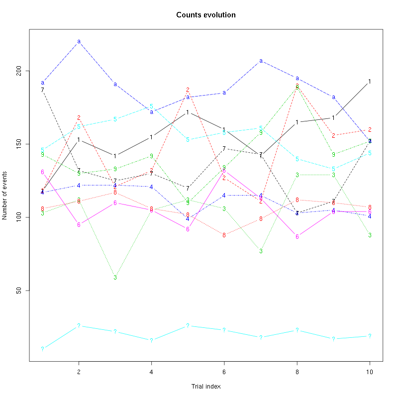
Figure 14: Evolution of the number of events attributed to each unit (1 to 9 plus "a") or unclassified ("?") during the 10 trials with Spontaneous 1 for tetrode D.

The waveform evolution is:

waveform_evolution(a_Spontaneous_1_tetD,threshold_factor,matrix(1:10,nr=5))

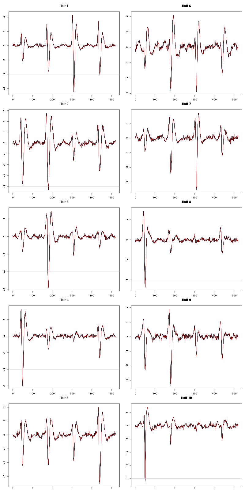
Figure 15: Evolution of the templates of each of the first five units during the 10 trials of Spontaneous 1 for tetrode D.

The observed counting processes and inter spike intervals densities for the first five units are:

cp_isi(a_Spontaneous_1_tetD,nbins=100)

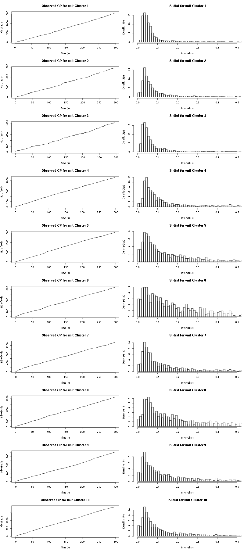
Figure 16: Observed counting processes and empirical inter spike interval distributions.

The BRT and RFT tests give for the first 7 units:

layout_matrix = matrix(0,nr=nbc-3,nc=nbc-3)
counter = 1
for (i in 1:(nbc-3))
    for (j in 1:(nbc-3))
        if (i != j) {
            layout_matrix[i,j] = counter
            counter = counter +1
        }
layout(layout_matrix)
par(mar=c(4,3,4,1))
for (i in 1:(nbc-3))
    for (j in 1:(nbc-3))
        if (i != j)
            test_rt(a_Spontaneous_1_tetD$spike_trains[[i]],
                    a_Spontaneous_1_tetD$spike_trains[[j]],
		    nbins=200, single_trial_duration=30,
                    ylab="",main=paste("Units",i,"and",j))

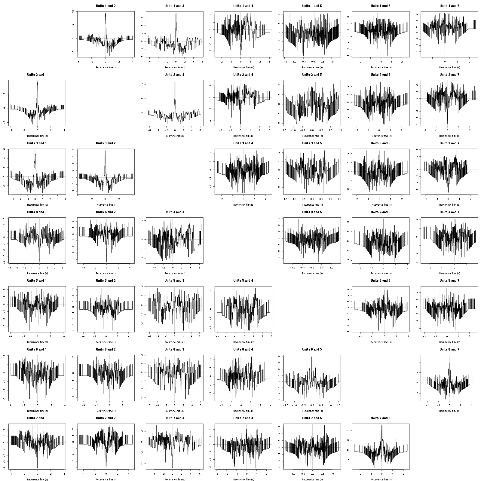
Figure 17: Graphical tests for the first 7 units of the Backward and Forward Reccurrence Times distribution against the null hypothesis (no interaction) during Spontaneous_1. If the null is correct, the curves should be IID draws from a standard normal distribution.

2.19.4 Save results

Before analyzing the next set of trials we save the output of sort_many_trials to disk with:

save(a_Spontaneous_1_tetD,
     file=paste0("tetD_analysis/tetD_","Spontaneous_1","_summary_obj.rda"))

We write to disk the spike trains in text mode:

for (c_idx in 1:length(a_Spontaneous_1_tetD$spike_trains))
    cat(a_Spontaneous_1_tetD$spike_trains[[c_idx]],
        file=paste0("locust20010217_spike_trains/locust20010217_Spontaneous_1_tetD_u",c_idx,".txt"),sep="\n")

2.20 Systematic analysis of the first 25 trials from `Spontaneous 3`

The description of the data states that the 10 trials of Spontaneous 2 had to be interrupted after the second one due to a fire alarm, so we go directly to the 30 trials of Spontaneous 3. There is moreover a noise problem (not mentioned in the lab book!!!) at trials 26, 27 and 28, so we stop at trial 25. To save space we do not print the output of the running code in the html document.

a_Spontaneous_3_tetD=sort_many_trials(inter_trial_time=30*15000,
                                      get_data_fct=function(i,s) get_data(i,s,
                                                                          channels = c("ch10","ch12","ch14","ch15"),
                                                                          file="locust20010217.hdf5"),
                                      stim_name="Spontaneous 3",
                                      trial_nbs=1:25,
                                      centers=a_Spontaneous_1_tetD$centers,
                                      counts=a_Spontaneous_1_tetD$counts,
                                      all_at_once_call_list=list(thres=threshold_factor*c(1,1,1,1), 
                                                                 filter_length_1=filter_length, filter_length=filter_length, 
                                                                 minimalDist_1=15, minimalDist=15, 
                                                                 before=c_before, after=c_after, 
                                                                 detection_cycle=c(0,0), verbose=1),
                                      layout_matrix=matrix(c(1,1:11),nr=6),new_weight_in_update=0.01
                                      )

2.20.1 Diagnostic plots

The counts evolution is:

counts_evolution(a_Spontaneous_3_tetD)

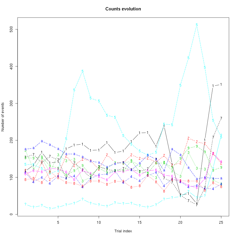
Figure 18: Evolution of the number of events attributed to each unit (1 to 9 plus "a") or unclassified ("?") during the 25 trials with Spontaneous 3 for tetrode D.

The waveform evolution is:

waveform_evolution(a_Spontaneous_3_tetD,threshold_factor,matrix(1:10,nr=5))

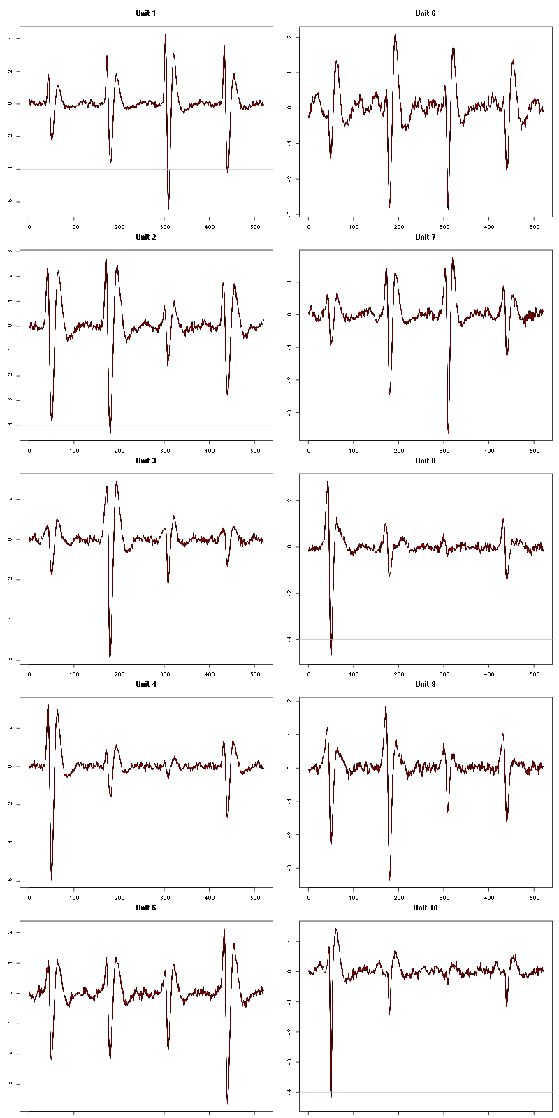
Figure 19: Evolution of the templates of each of the first five units during the 25 trials of Spontaneous 3 for tetrode D.

The observed counting processes and inter spike intervals densities are:

cp_isi(a_Spontaneous_3_tetD,nbins=100)

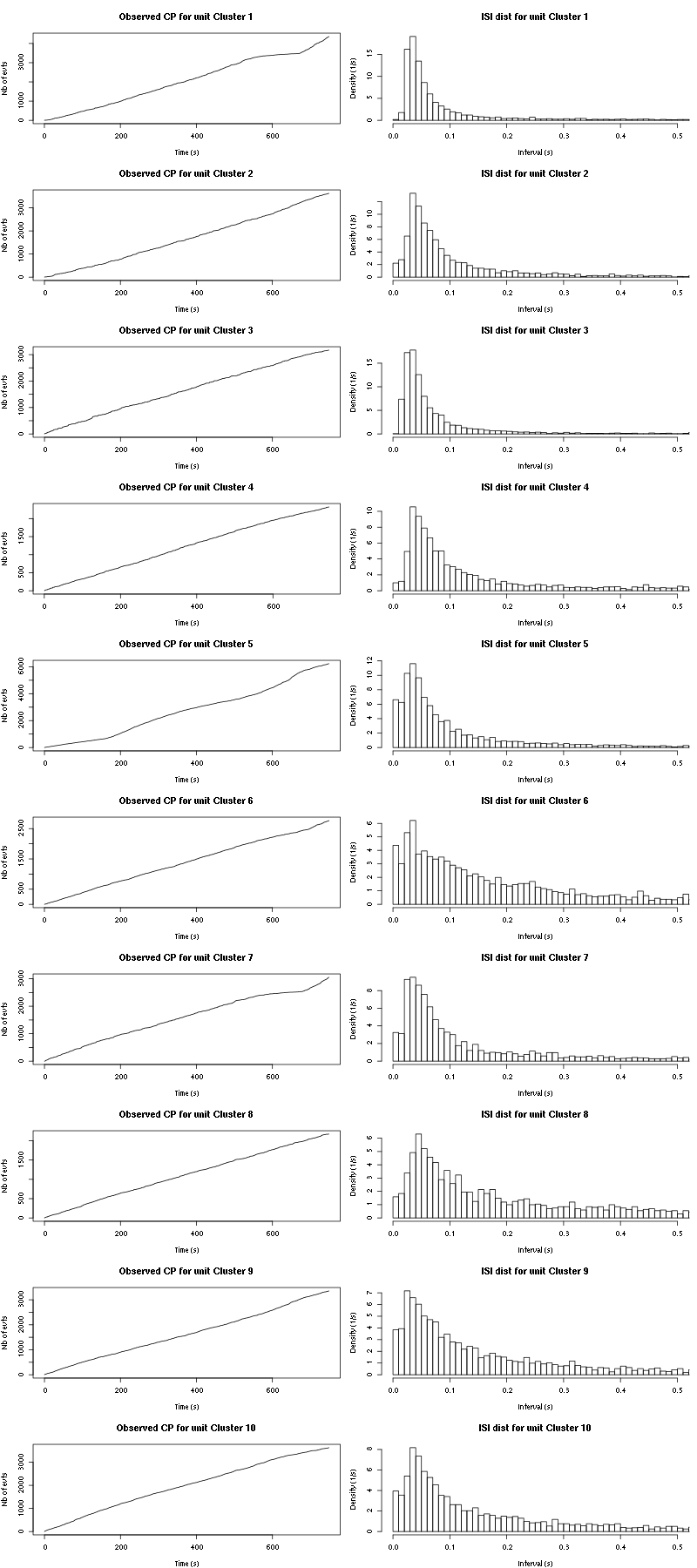
Figure 20: Observed counting processes and empirical inter spike interval distributions.

The BRT and RFT tests give for the first 7 units:

layout_matrix = matrix(0,nr=nbc-3,nc=nbc-3)
counter = 1
for (i in 1:(nbc-3))
    for (j in 1:(nbc-3))
        if (i != j) {
            layout_matrix[i,j] = counter
            counter = counter +1
        }
layout(layout_matrix)
par(mar=c(4,3,4,1))
for (i in 1:(nbc-3))
    for (j in 1:(nbc-3))
        if (i != j)
            test_rt(a_Spontaneous_3_tetD$spike_trains[[i]],
                    a_Spontaneous_3_tetD$spike_trains[[j]],
		    nbins=500, single_trial_duration=30,
                    ylab="",main=paste("Units",i,"and",j),
                    xlim=c(-0.1,0.1))

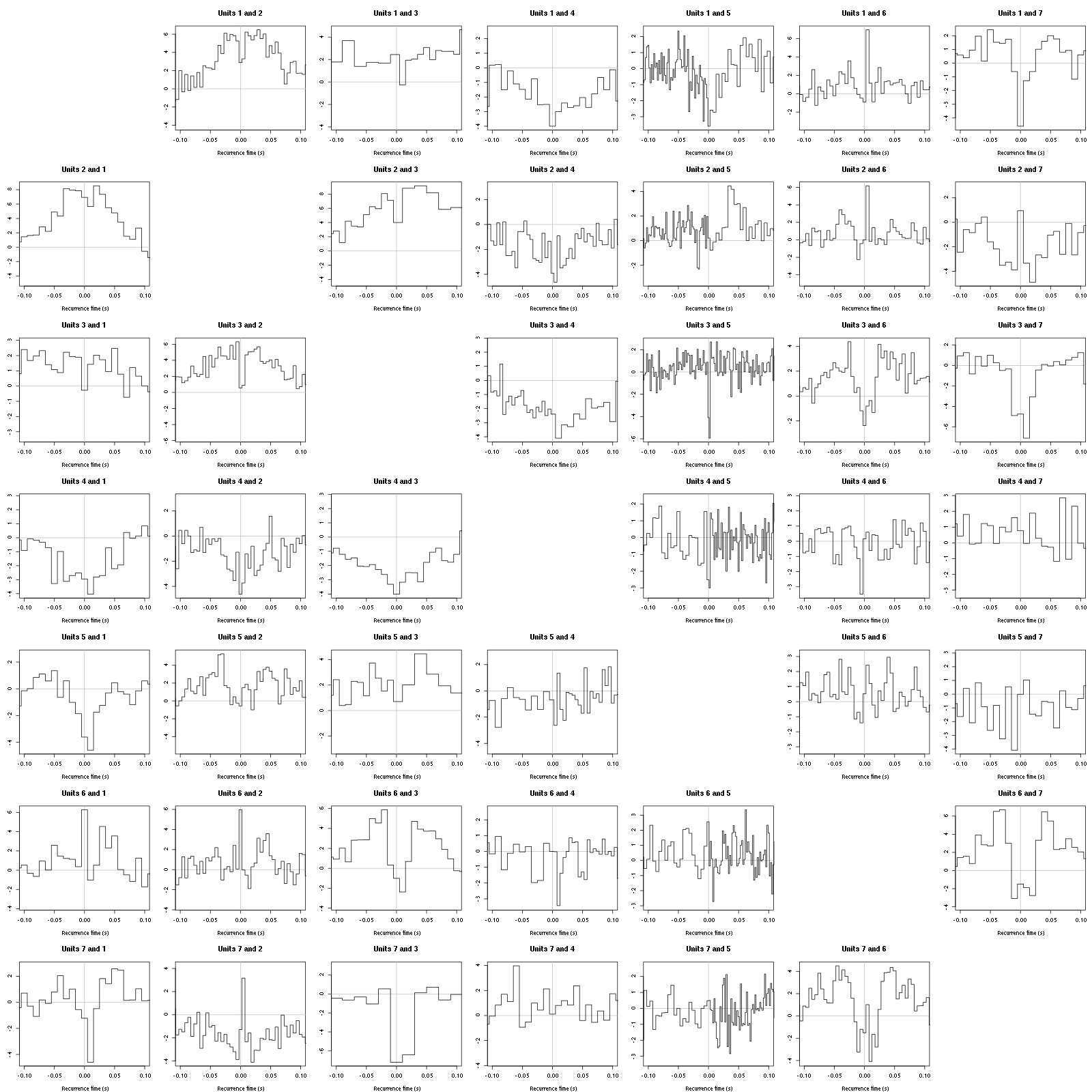
Figure 21: Graphical tests for the first 7 units of the Backward and Forward Reccurrence Times distribution against the null hypothesis (no interaction) during Spontaneous_3. If the null is correct, the curves should be IID draws from a standard normal distribution.

2.20.2 Save results

Before analyzing the next set of trials we save the output of sort_many_trials to disk with:

save(a_Spontaneous_3_tetD,
     file=paste0("tetD_analysis/tetD_","Spontaneous_3","_summary_obj.rda"))

We write to disk the spike trains in text mode:

for (c_idx in 1:length(a_Spontaneous_3_tetD$spike_trains))
    cat(a_Spontaneous_3_tetD$spike_trains[[c_idx]],
        file=paste0("locust20010217_spike_trains/locust20010217_Spontaneous_3_tetD_u",c_idx,".txt"),sep="\n")

2.21 Systematic analysis of the 10 trials from `Spontaneous 4`

a_Spontaneous_4_tetD=sort_many_trials(inter_trial_time=30*15000,
                                      get_data_fct=function(i,s) get_data(i,s,
                                                                          channels = c("ch10","ch12","ch14","ch15"),
                                                                          file="locust20010217.hdf5"),
                                      stim_name="Spontaneous 4",
                                      trial_nbs=1:10,
                                      centers=a_Spontaneous_3_tetD$centers,
                                      counts=a_Spontaneous_3_tetD$counts,
                                      all_at_once_call_list=list(thres=threshold_factor*c(1,1,1,1), 
                                                                 filter_length_1=filter_length, filter_length=filter_length, 
                                                                 minimalDist_1=15, minimalDist=15, 
                                                                 before=c_before, after=c_after, 
                                                                 detection_cycle=c(0,0), verbose=1),
                                      layout_matrix=matrix(c(1,1:11),nr=6),new_weight_in_update=0.01
                                      )

2.21.1 Diagnostic plots

The counts evolution is:

counts_evolution(a_Spontaneous_4_tetD)

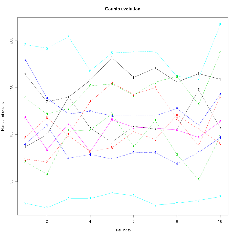
Figure 22: Evolution of the number of events attributed to each unit (1 to 9 plus "a") or unclassified ("?") during the 10 trials with Spontaneous 4 for tetrode D.

The waveform evolution is:

waveform_evolution(a_Spontaneous_4_tetD,threshold_factor,matrix(1:10,nr=5))

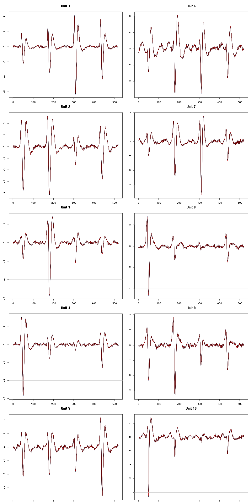
Figure 23: Evolution of the templates of each of the first five units during the 10 trials of Spontaneous 4 for tetrode D.

The observed counting processes and inter spike intervals densities are:

cp_isi(a_Spontaneous_4_tetD,nbins=100)

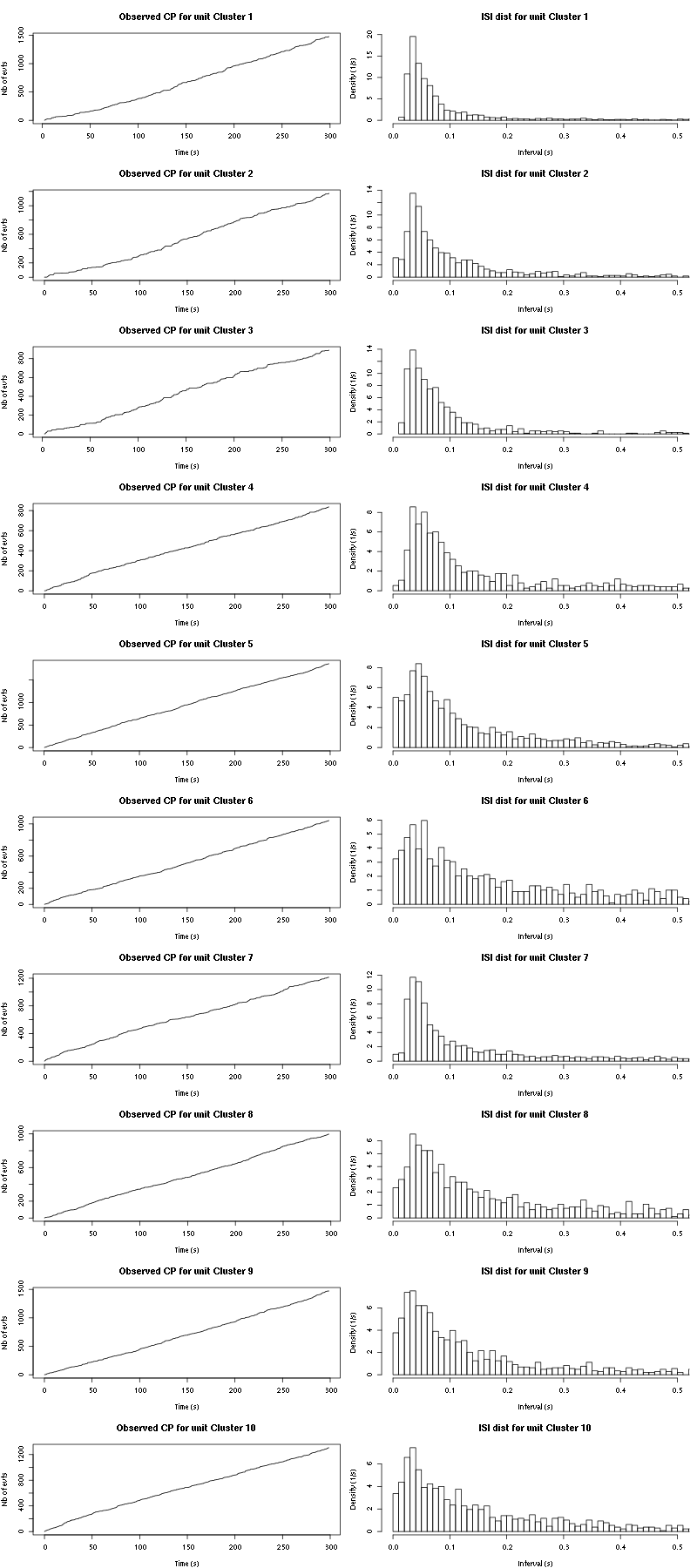
Figure 24: Observed counting processes and empirical inter spike interval distributions.

The BRT and RFT tests give for the first 7 units:

layout_matrix = matrix(0,nr=nbc-3,nc=nbc-3)
counter = 1
for (i in 1:(nbc-3))
    for (j in 1:(nbc-3))
        if (i != j) {
            layout_matrix[i,j] = counter
            counter = counter +1
        }
layout(layout_matrix)
par(mar=c(4,3,4,1))
for (i in 1:(nbc-3))
    for (j in 1:(nbc-3))
        if (i != j)
            test_rt(a_Spontaneous_4_tetD$spike_trains[[i]],
                    a_Spontaneous_4_tetD$spike_trains[[j]],
		    nbins=200, single_trial_duration=30,
                    ylab="",main=paste("Units",i,"and",j),
                    xlim=c(-0.1,0.1))

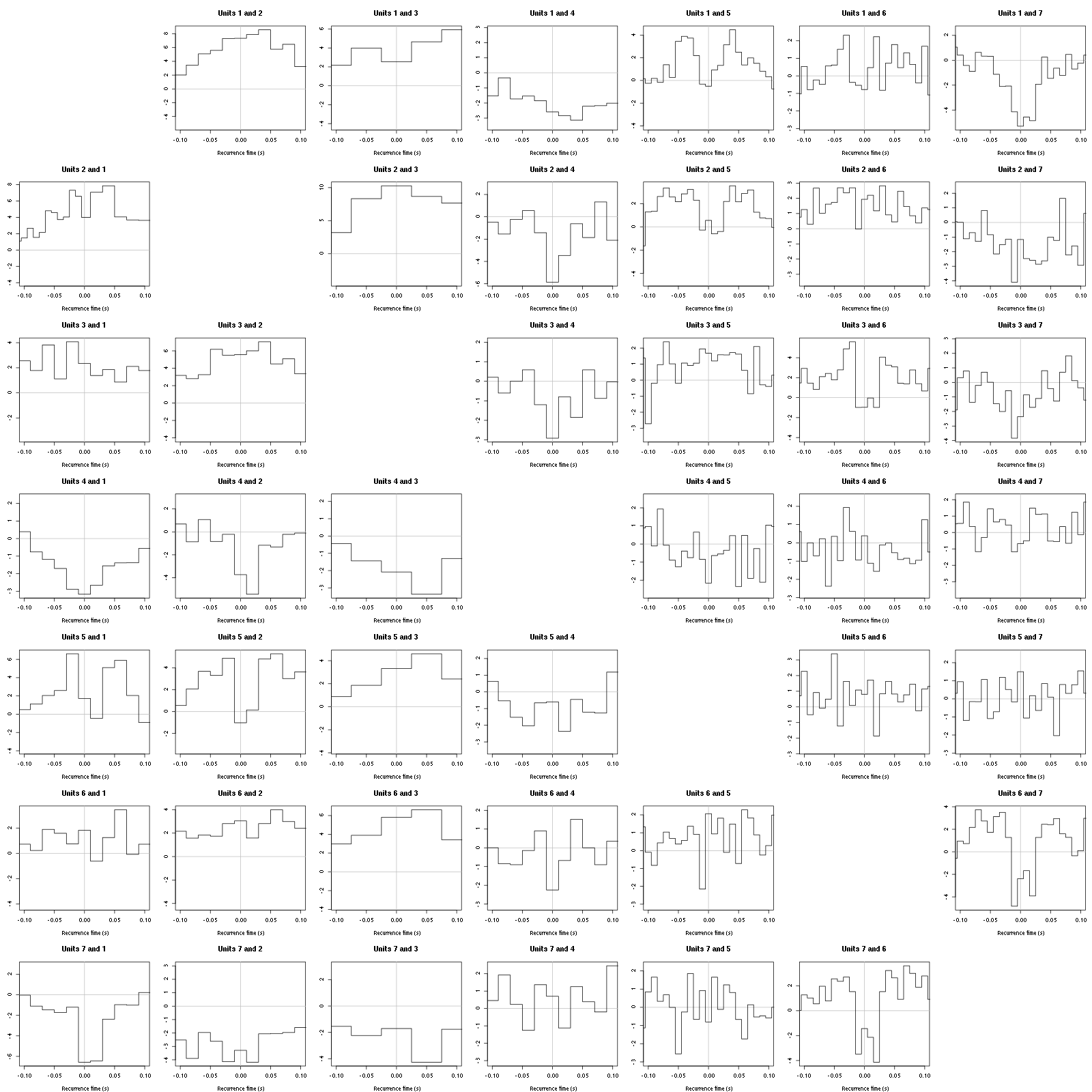
Figure 25: Graphical tests for the first 7 units of the Backward and Forward Reccurrence Times distribution against the null hypothesis (no interaction) during Spontaneous_4. If the null is correct, the curves should be IID draws from a standard normal distribution.

2.21.2 Save results

Before analyzing the next set of trials we save the output of sort_many_trials to disk with:

save(a_Spontaneous_4_tetD,
     file=paste0("tetD_analysis/tetD_","Spontaneous_4","_summary_obj.rda"))

We write to disk the spike trains in text mode:

for (c_idx in 1:length(a_Spontaneous_4_tetD$spike_trains))
    cat(a_Spontaneous_4_tetD$spike_trains[[c_idx]],
        file=paste0("locust20010217_spike_trains/locust20010217_Spontaneous_4_tetD_u",c_idx,".txt"),sep="\n")

2.22 Systematic analysis of the 10 trials from `Spontaneous 5`

a_Spontaneous_5_tetD=sort_many_trials(inter_trial_time=30*15000,
                                      get_data_fct=function(i,s) get_data(i,s,
                                                                          channels = c("ch10","ch12","ch14","ch15"),
                                                                          file="locust20010217.hdf5"),
                                      stim_name="Spontaneous 5",
                                      trial_nbs=1:10,
                                      centers=a_Spontaneous_4_tetD$centers,
                                      counts=a_Spontaneous_4_tetD$counts,
                                      all_at_once_call_list=list(thres=threshold_factor*c(1,1,1,1), 
                                                                 filter_length_1=filter_length, filter_length=filter_length, 
                                                                 minimalDist_1=15, minimalDist=15, 
                                                                 before=c_before, after=c_after, 
                                                                 detection_cycle=c(0,0), verbose=1),
                                      layout_matrix=matrix(c(1,1:11),nr=6),new_weight_in_update=0.01
                                      )

2.22.1 Diagnostic plots

The counts evolution is:

counts_evolution(a_Spontaneous_5_tetD)

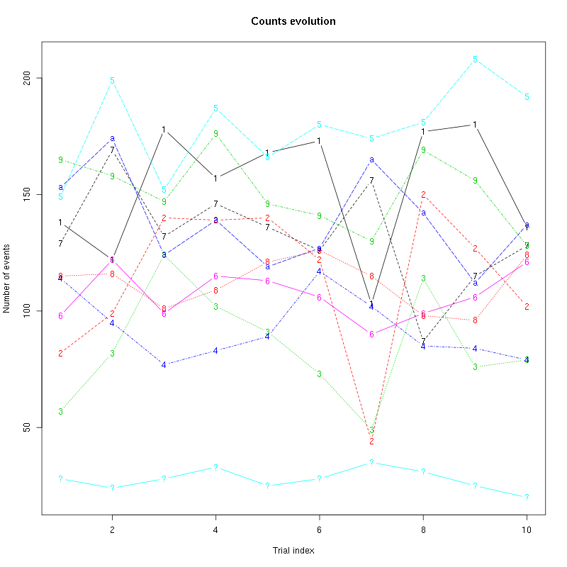
Figure 26: Evolution of the number of events attributed to each unit (1 to 9 plus "a") or unclassified ("?") during the 10 trials with Spontaneous 5 for tetrode D.

The waveform evolution is:

waveform_evolution(a_Spontaneous_5_tetD,threshold_factor,matrix(1:10,nr=5))

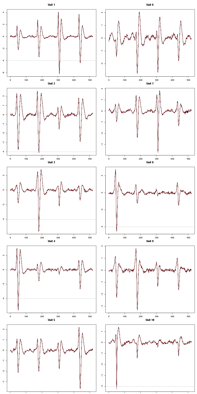
Figure 27: Evolution of the templates of each of the first five units during the 10 trials of Spontaneous 5 for tetrode D.

The observed counting processes and inter spike intervals densities are:

cp_isi(a_Spontaneous_5_tetD,nbins=100)

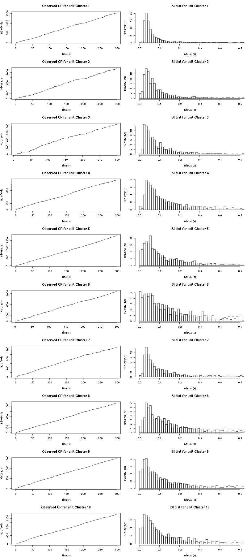
Figure 28: Observed counting processes and empirical inter spike interval distributions.

The BRT and RFT tests give for the first 7 units:

layout_matrix = matrix(0,nr=nbc-3,nc=nbc-3)
counter = 1
for (i in 1:(nbc-3))
    for (j in 1:(nbc-3))
        if (i != j) {
            layout_matrix[i,j] = counter
            counter = counter +1
        }
layout(layout_matrix)
par(mar=c(4,3,4,1))
for (i in 1:(nbc-3))
    for (j in 1:(nbc-3))
        if (i != j)
            test_rt(a_Spontaneous_5_tetD$spike_trains[[i]],
                    a_Spontaneous_5_tetD$spike_trains[[j]],
		    nbins=200, single_trial_duration=30,
                    ylab="",main=paste("Units",i,"and",j),
                    xlim=c(-0.1,0.1))

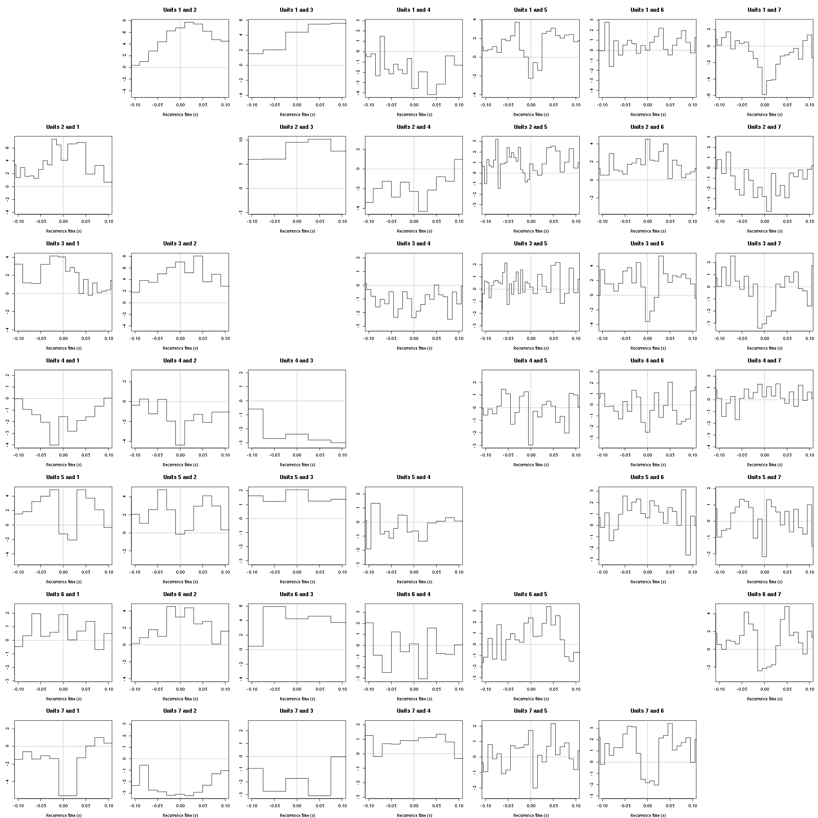
Figure 29: Graphical tests for the first 7 units of the Backward and Forward Reccurrence Times distribution against the null hypothesis (no interaction) during Spontaneous_5. If the null is correct, the curves should be IID draws from a standard normal distribution.

2.22.2 Save results

Before analyzing the next set of trials we save the output of sort_many_trials to disk with:

save(a_Spontaneous_5_tetD,
     file=paste0("tetD_analysis/tetD_","Spontaneous_5","_summary_obj.rda"))

We write to disk the spike trains in text mode:

for (c_idx in 1:length(a_Spontaneous_5_tetD$spike_trains))
    cat(a_Spontaneous_5_tetD$spike_trains[[c_idx]],
        file=paste0("locust20010217_spike_trains/locust20010217_Spontaneous_5_tetD_u",c_idx,".txt"),sep="\n")

2.23 Systematic analysis of the 10 trials from `Spontaneous 6`

a_Spontaneous_6_tetD=sort_many_trials(inter_trial_time=30*15000,
                                      get_data_fct=function(i,s) get_data(i,s,
                                                                          channels = c("ch10","ch12","ch14","ch15"),
                                                                          file="locust20010217.hdf5"),
                                      stim_name="Spontaneous 6",
                                      trial_nbs=1:10,
                                      centers=a_Spontaneous_5_tetD$centers,
                                      counts=a_Spontaneous_5_tetD$counts,
                                      all_at_once_call_list=list(thres=threshold_factor*c(1,1,1,1), 
                                                                 filter_length_1=filter_length, filter_length=filter_length, 
                                                                 minimalDist_1=15, minimalDist=15, 
                                                                 before=c_before, after=c_after, 
                                                                 detection_cycle=c(0,0), verbose=1),
                                      layout_matrix=matrix(c(1,1:11),nr=6),new_weight_in_update=0.01
                                      )

2.23.1 Diagnostic plots

The counts evolution is:

counts_evolution(a_Spontaneous_6_tetD)

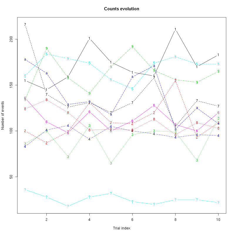
Figure 30: Evolution of the number of events attributed to each unit (1 to 9 plus "a") or unclassified ("?") during the 10 trials with Spontaneous 6 for tetrode D.

The waveform evolution is:

waveform_evolution(a_Spontaneous_6_tetD,threshold_factor,matrix(1:10,nr=5))

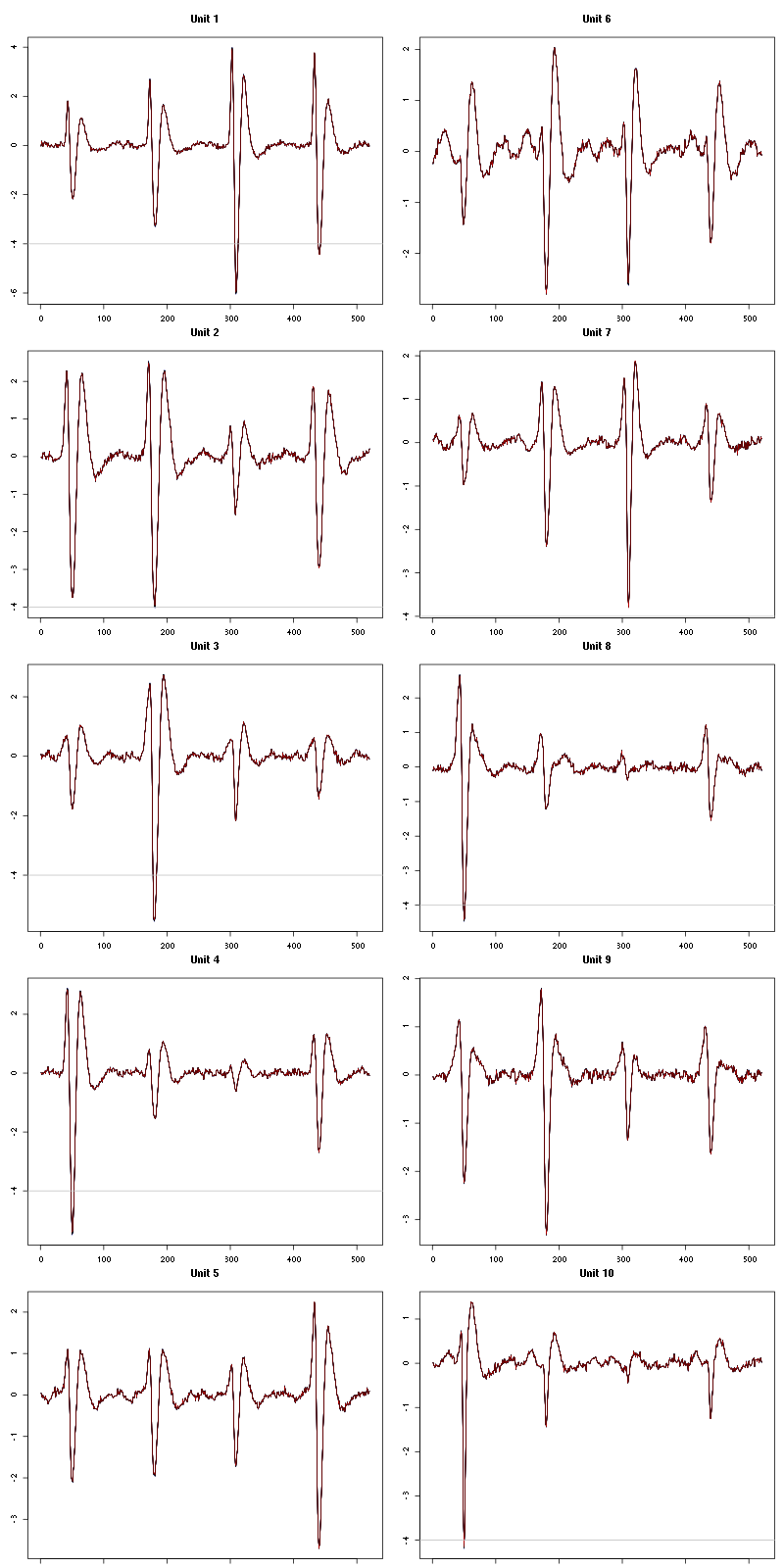
Figure 31: Evolution of the templates of each of the first five units during the 10 trials of Spontaneous 6 for tetrode D.

The observed counting processes and inter spike intervals densities are:

cp_isi(a_Spontaneous_6_tetD,nbins=100)

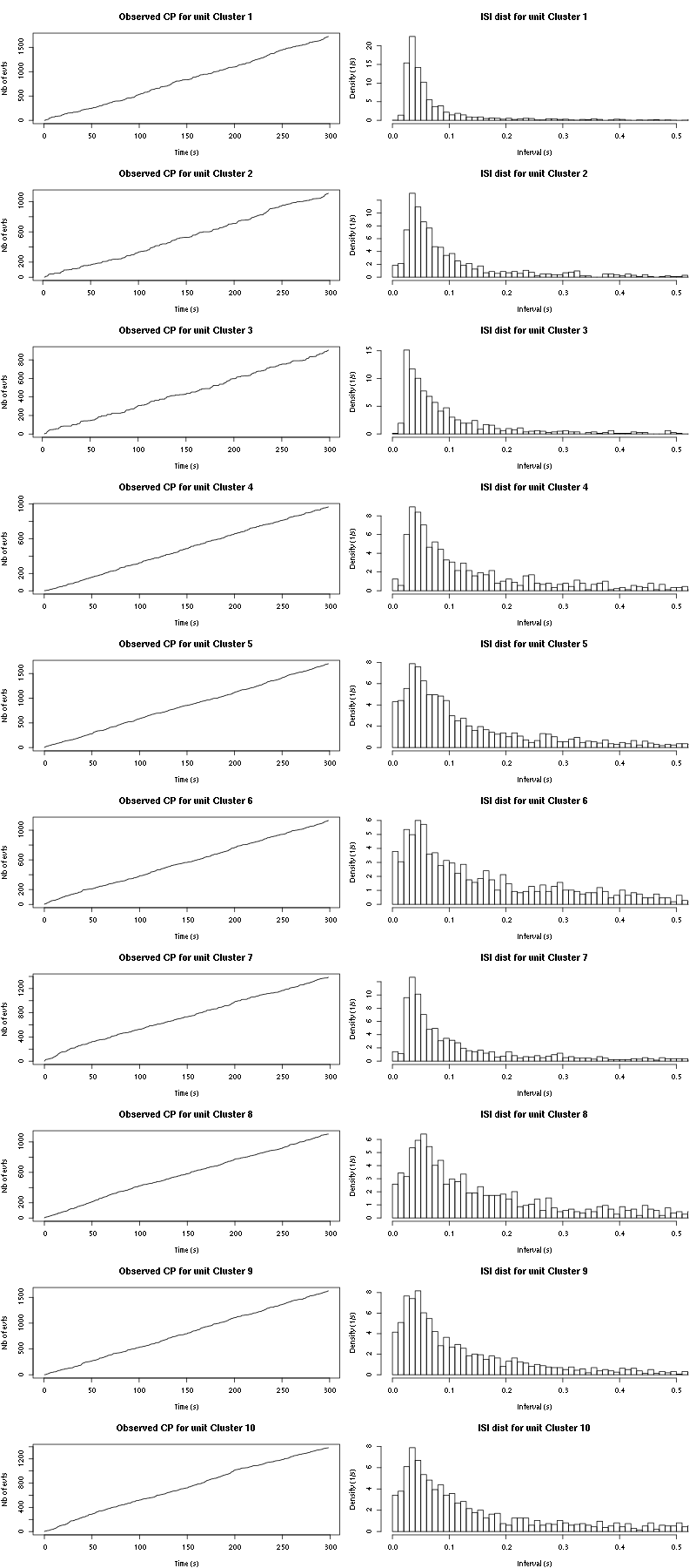
Figure 32: Observed counting processes and empirical inter spike interval distributions.

The BRT and RFT tests give for the first 7 units:

layout_matrix = matrix(0,nr=nbc-3,nc=nbc-3)
counter = 1
for (i in 1:(nbc-3))
    for (j in 1:(nbc-3))
        if (i != j) {
            layout_matrix[i,j] = counter
            counter = counter +1
        }
layout(layout_matrix)
par(mar=c(4,3,4,1))
for (i in 1:(nbc-3))
    for (j in 1:(nbc-3))
        if (i != j)
            test_rt(a_Spontaneous_6_tetD$spike_trains[[i]],
                    a_Spontaneous_6_tetD$spike_trains[[j]],
		    nbins=200, single_trial_duration=30,
                    ylab="",main=paste("Units",i,"and",j),
                    xlim=c(-0.1,0.1))

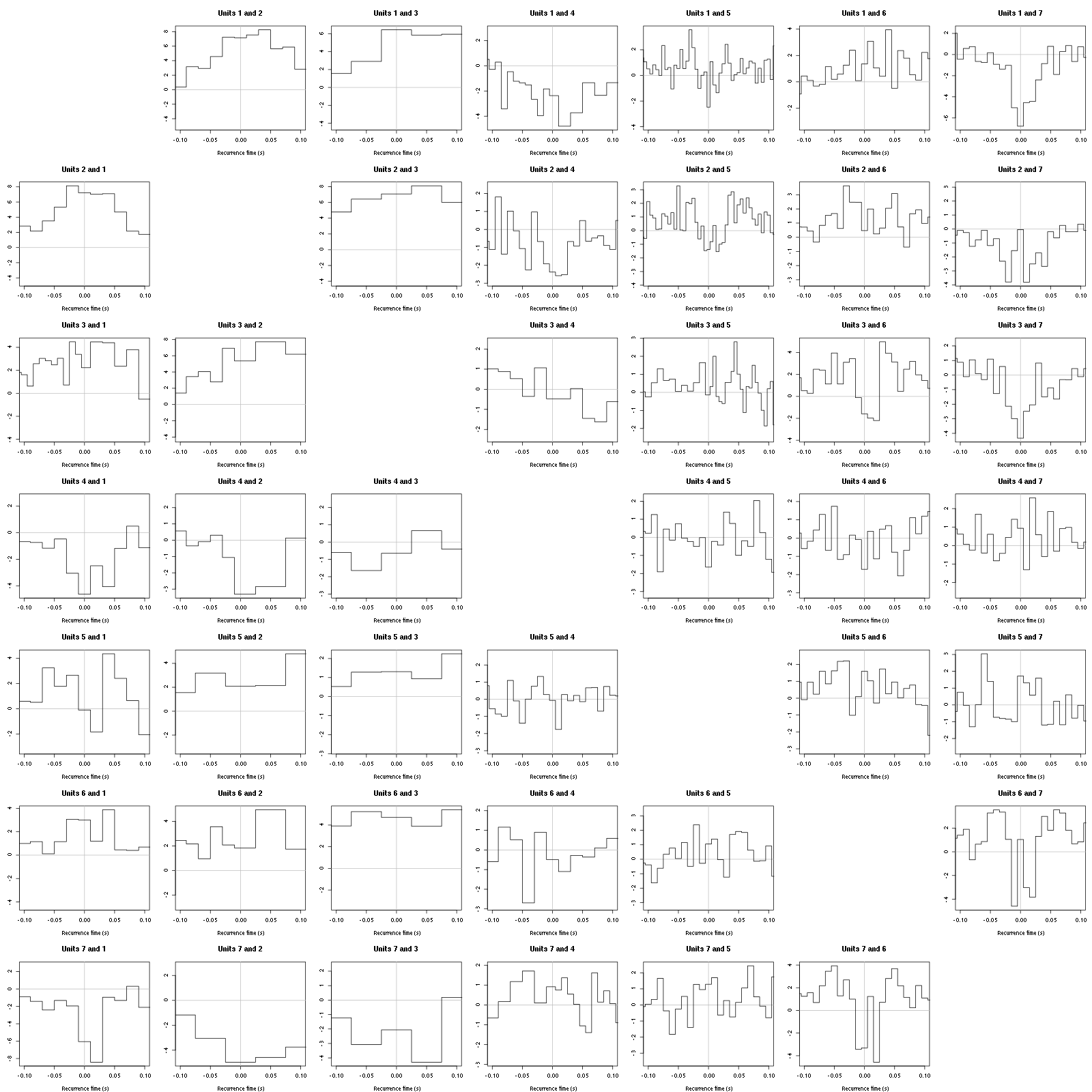
Figure 33: Graphical tests for the first 7 units of the Backward and Forward Reccurrence Times distribution against the null hypothesis (no interaction) during Spontaneous_6. If the null is correct, the curves should be IID draws from a standard normal distribution.

2.23.2 Save results

Before analyzing the next set of trials we save the output of sort_many_trials to disk with:

save(a_Spontaneous_6_tetD,
     file=paste0("tetD_analysis/tetD_","Spontaneous_6","_summary_obj.rda"))

We write to disk the spike trains in text mode:

for (c_idx in 1:length(a_Spontaneous_6_tetD$spike_trains))
    cat(a_Spontaneous_6_tetD$spike_trains[[c_idx]],
        file=paste0("locust20010217_spike_trains/locust20010217_Spontaneous_6_tetD_u",c_idx,".txt"),sep="\n")

2.24 Systematic analysis of the 10 trials from `Spontaneous 7`

a_Spontaneous_7_tetD=sort_many_trials(inter_trial_time=30*15000,
                                      get_data_fct=function(i,s) get_data(i,s,
                                                                          channels = c("ch10","ch12","ch14","ch15"),
                                                                          file="locust20010217.hdf5"),
                                      stim_name="Spontaneous 7",
                                      trial_nbs=1:10,
                                      centers=a_Spontaneous_6_tetD$centers,
                                      counts=a_Spontaneous_6_tetD$counts,
                                      all_at_once_call_list=list(thres=threshold_factor*c(1,1,1,1), 
                                                                 filter_length_1=filter_length, filter_length=filter_length, 
                                                                 minimalDist_1=15, minimalDist=15, 
                                                                 before=c_before, after=c_after, 
                                                                 detection_cycle=c(0,0), verbose=1),
                                      layout_matrix=matrix(c(1,1:11),nr=6),new_weight_in_update=0.01
                                      )

2.24.1 Diagnostic plots

The counts evolution is:

counts_evolution(a_Spontaneous_7_tetD)

Figure 34: Evolution of the number of events attributed to each unit (1 to 9 plus "a") or unclassified ("?") during the 10 trials with Spontaneous 7 for tetrode D.

The waveform evolution is:

waveform_evolution(a_Spontaneous_7_tetD,threshold_factor,matrix(1:10,nr=5))

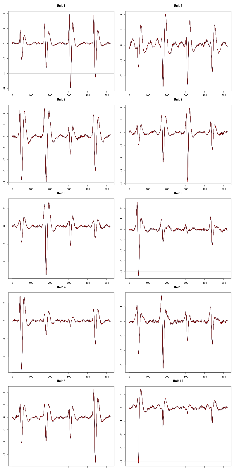
Figure 35: Evolution of the templates of each of the first five units during the 10 trials of Spontaneous 7 for tetrode D.

The observed counting processes and inter spike intervals densities are:

cp_isi(a_Spontaneous_7_tetD,nbins=100)

Figure 36: Observed counting processes and empirical inter spike interval distributions.

The BRT and RFT tests give for the first 7 units:

layout_matrix = matrix(0,nr=nbc-3,nc=nbc-3)
counter = 1
for (i in 1:(nbc-3))
    for (j in 1:(nbc-3))
        if (i != j) {
            layout_matrix[i,j] = counter
            counter = counter +1
        }
layout(layout_matrix)
par(mar=c(4,3,4,1))
for (i in 1:(nbc-3))
    for (j in 1:(nbc-3))
        if (i != j)
            test_rt(a_Spontaneous_7_tetD$spike_trains[[i]],
                    a_Spontaneous_7_tetD$spike_trains[[j]],
		    nbins=200, single_trial_duration=30,
                    ylab="",main=paste("Units",i,"and",j),
                    xlim=c(-0.1,0.1))

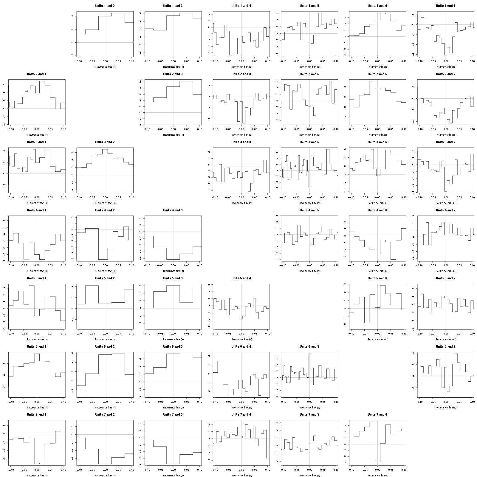
Figure 37: Graphical tests for the first 7 units of the Backward and Forward Reccurrence Times distribution against the null hypothesis (no interaction) during Spontaneous_7. If the null is correct, the curves should be IID draws from a standard normal distribution.

2.24.2 Save results

Before analyzing the next set of trials we save the output of sort_many_trials to disk with:

save(a_Spontaneous_7_tetD,
     file=paste0("tetD_analysis/tetD_","Spontaneous_7","_summary_obj.rda"))

We write to disk the spike trains in text mode:

for (c_idx in 1:length(a_Spontaneous_7_tetD$spike_trains))
    cat(a_Spontaneous_7_tetD$spike_trains[[c_idx]],
        file=paste0("locust20010217_spike_trains/locust20010217_Spontaneous_7_tetD_u",c_idx,".txt"),sep="\n")

2.25 Systematic analysis of the 10 trials from `Spontaneous 8`

a_Spontaneous_8_tetD=sort_many_trials(inter_trial_time=30*15000,
                                      get_data_fct=function(i,s) get_data(i,s,
                                                                          channels = c("ch10","ch12","ch14","ch15"),
                                                                          file="locust20010217.hdf5"),
                                      stim_name="Spontaneous 8",
                                      trial_nbs=1:10,
                                      centers=a_Spontaneous_7_tetD$centers,
                                      counts=a_Spontaneous_7_tetD$counts,
                                      all_at_once_call_list=list(thres=threshold_factor*c(1,1,1,1), 
                                                                 filter_length_1=filter_length, filter_length=filter_length, 
                                                                 minimalDist_1=15, minimalDist=15, 
                                                                 before=c_before, after=c_after, 
                                                                 detection_cycle=c(0,0), verbose=1),
                                      layout_matrix=matrix(c(1,1:11),nr=6),new_weight_in_update=0.01
                                      )

2.25.1 Diagnostic plots

The counts evolution is:

counts_evolution(a_Spontaneous_8_tetD)

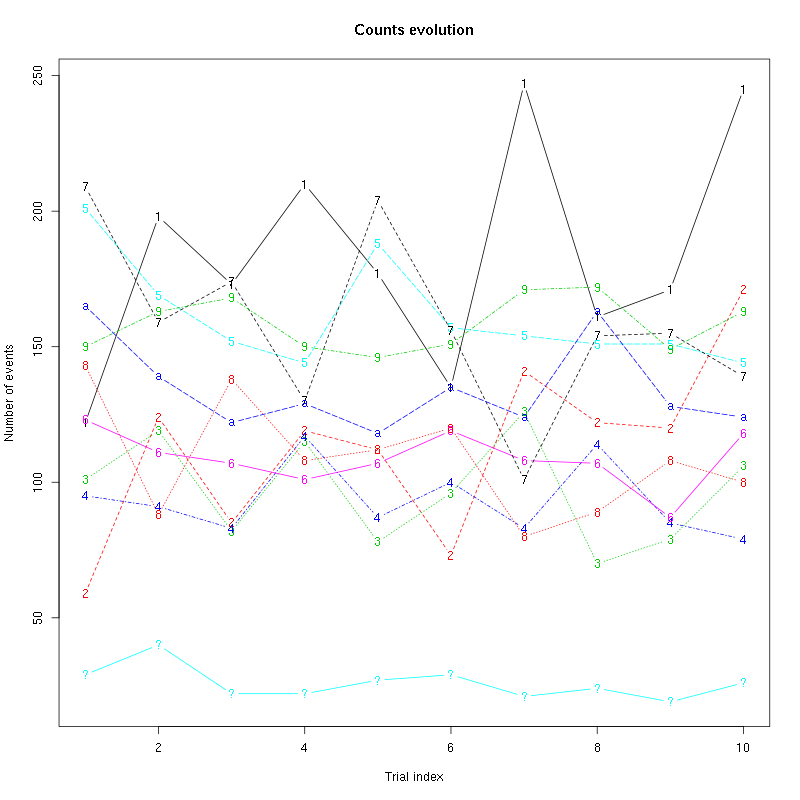
Figure 38: Evolution of the number of events attributed to each unit (1 to 9 plus "a") or unclassified ("?") during the 10 trials with Spontaneous 8 for tetrode D.

The waveform evolution is:

waveform_evolution(a_Spontaneous_8_tetD,threshold_factor,matrix(1:10,nr=5))

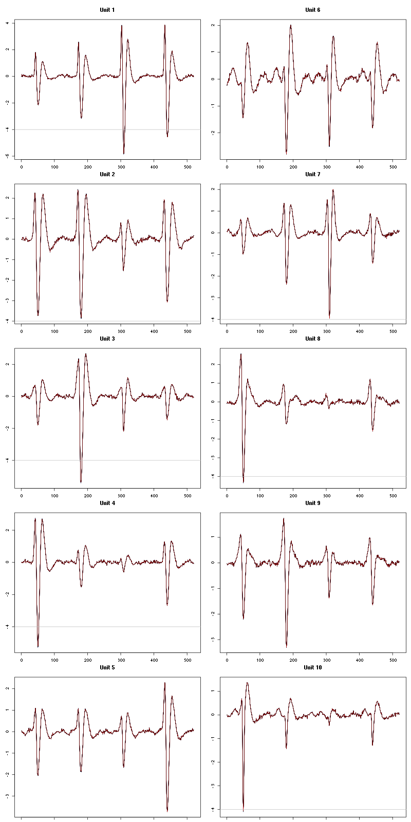
Figure 39: Evolution of the templates of each of the first five units during the 10 trials of Spontaneous 8 for tetrode D.

The observed counting processes and inter spike intervals densities are:

cp_isi(a_Spontaneous_8_tetD,nbins=100)

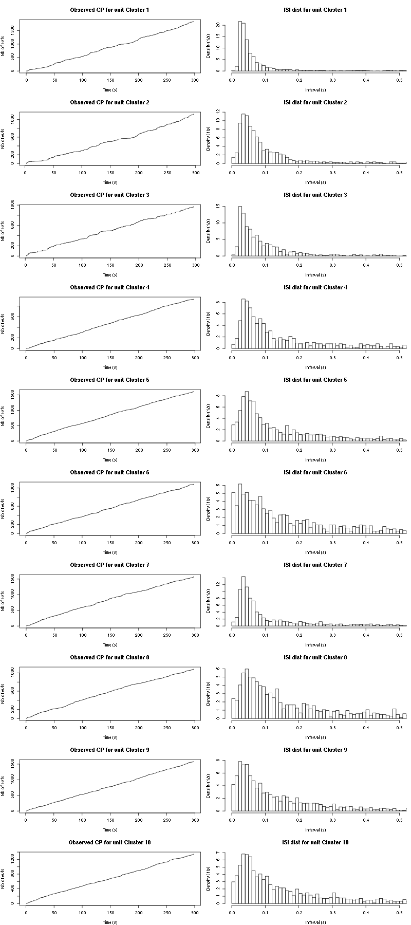
Figure 40: Observed counting processes and empirical inter spike interval distributions.

The BRT and RFT tests give for the first 7 units:

layout_matrix = matrix(0,nr=nbc-3,nc=nbc-3)
counter = 1
for (i in 1:(nbc-3))
    for (j in 1:(nbc-3))
        if (i != j) {
            layout_matrix[i,j] = counter
            counter = counter +1
        }
layout(layout_matrix)
par(mar=c(4,3,4,1))
for (i in 1:(nbc-3))
    for (j in 1:(nbc-3))
        if (i != j)
            test_rt(a_Spontaneous_8_tetD$spike_trains[[i]],
                    a_Spontaneous_8_tetD$spike_trains[[j]],
		    nbins=200, single_trial_duration=30,
                    ylab="",main=paste("Units",i,"and",j),
                    xlim=c(-0.1,0.1))

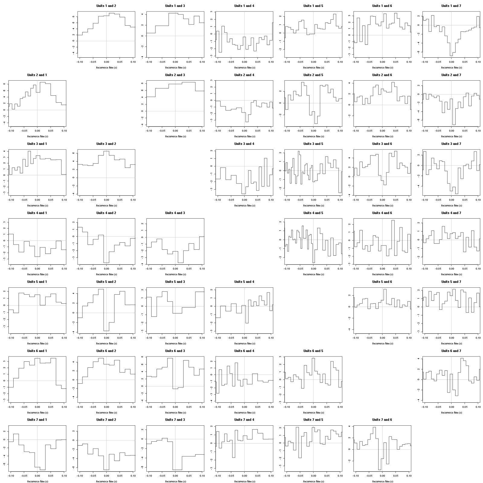
Figure 41: Graphical tests for the first 7 units of the Backward and Forward Reccurrence Times distribution against the null hypothesis (no interaction) during Spontaneous_8. If the null is correct, the curves should be IID draws from a standard normal distribution.

2.25.2 Save results

Before analyzing the next set of trials we save the output of sort_many_trials to disk with:

save(a_Spontaneous_8_tetD,
     file=paste0("tetD_analysis/tetD_","Spontaneous_8","_summary_obj.rda"))

We write to disk the spike trains in text mode:

for (c_idx in 1:length(a_Spontaneous_8_tetD$spike_trains))
    cat(a_Spontaneous_8_tetD$spike_trains[[c_idx]],
        file=paste0("locust20010217_spike_trains/locust20010217_Spontaneous_8_tetD_u",c_idx,".txt"),sep="\n")

2.26 Systematic analysis of the 10 trials from `Spontaneous 9`

a_Spontaneous_9_tetD=sort_many_trials(inter_trial_time=30*15000,
                                      get_data_fct=function(i,s) get_data(i,s,
                                                                          channels = c("ch10","ch12","ch14","ch15"),
                                                                          file="locust20010217.hdf5"),
                                      stim_name="Spontaneous 9",
                                      trial_nbs=1:10,
                                      centers=a_Spontaneous_8_tetD$centers,
                                      counts=a_Spontaneous_8_tetD$counts,
                                      all_at_once_call_list=list(thres=threshold_factor*c(1,1,1,1), 
                                                                 filter_length_1=filter_length, filter_length=filter_length, 
                                                                 minimalDist_1=15, minimalDist=15, 
                                                                 before=c_before, after=c_after, 
                                                                 detection_cycle=c(0,0), verbose=1),
                                      layout_matrix=matrix(c(1,1:11),nr=6),new_weight_in_update=0.01
                                      )

2.26.1 Diagnostic plots

The counts evolution is:

counts_evolution(a_Spontaneous_9_tetD)

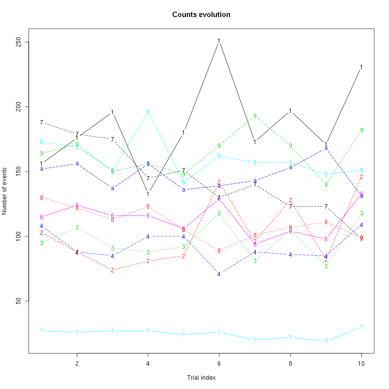
Figure 42: Evolution of the number of events attributed to each unit (1 to 9 plus "a") or unclassified ("?") during the 10 trials with Spontaneous 9 for tetrode D.

The waveform evolution is:

waveform_evolution(a_Spontaneous_9_tetD,threshold_factor,matrix(1:10,nr=5))

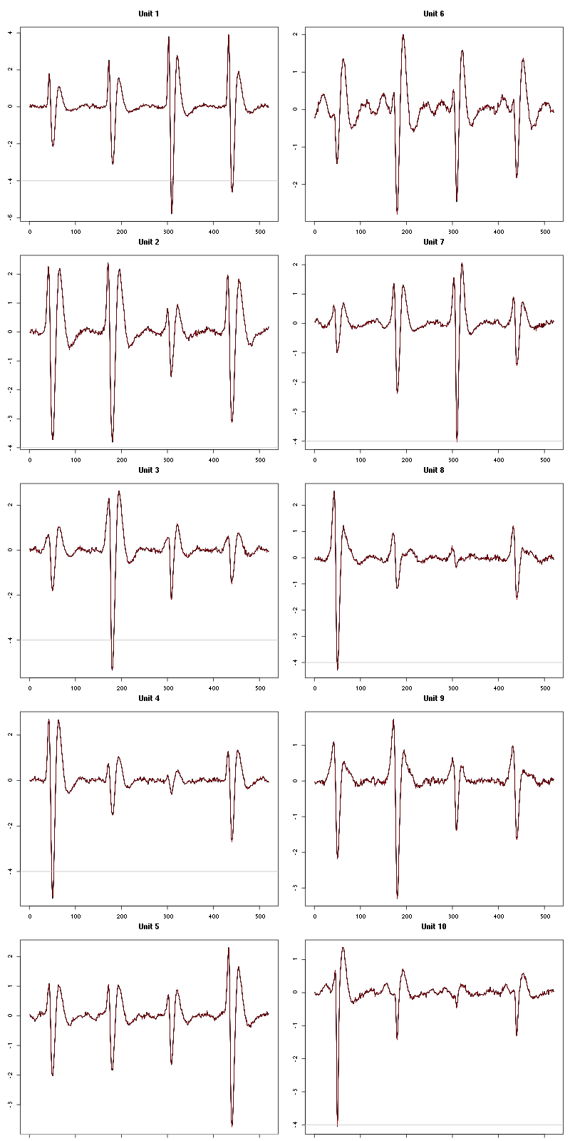
Figure 43: Evolution of the templates of each of the first five units during the 10 trials of Spontaneous 9 for tetrode D.

The observed counting processes and inter spike intervals densities are:

cp_isi(a_Spontaneous_9_tetD,nbins=100)

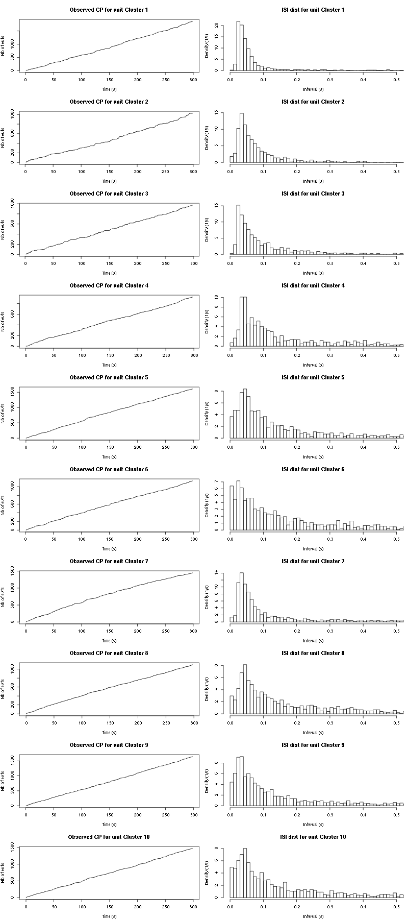
Figure 44: Observed counting processes and empirical inter spike interval distributions.

The BRT and RFT tests give for the first 7 units:

layout_matrix = matrix(0,nr=nbc-3,nc=nbc-3)
counter = 1
for (i in 1:(nbc-3))
    for (j in 1:(nbc-3))
        if (i != j) {
            layout_matrix[i,j] = counter
            counter = counter +1
        }
layout(layout_matrix)
par(mar=c(4,3,4,1))
for (i in 1:(nbc-3))
    for (j in 1:(nbc-3))
        if (i != j)
            test_rt(a_Spontaneous_9_tetD$spike_trains[[i]],
                    a_Spontaneous_9_tetD$spike_trains[[j]],
		    nbins=200, single_trial_duration=30,
                    ylab="",main=paste("Units",i,"and",j),
                    xlim=c(-0.1,0.1))

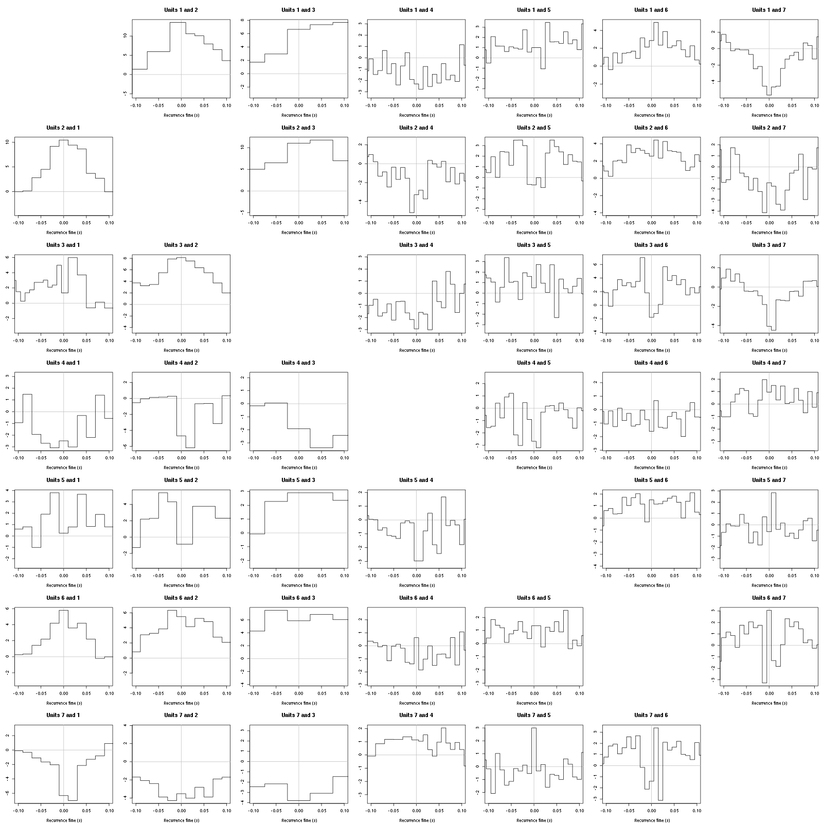
Figure 45: Graphical tests for the first 7 units of the Backward and Forward Reccurrence Times distribution against the null hypothesis (no interaction) during Spontaneous_9. If the null is correct, the curves should be IID draws from a standard normal distribution.

2.26.2 Save results

Before analyzing the next set of trials we save the output of sort_many_trials to disk with:

save(a_Spontaneous_9_tetD,
     file=paste0("tetD_analysis/tetD_","Spontaneous_9","_summary_obj.rda"))

We write to disk the spike trains in text mode:

for (c_idx in 1:length(a_Spontaneous_9_tetD$spike_trains))
    cat(a_Spontaneous_9_tetD$spike_trains[[c_idx]],
        file=paste0("locust20010217_spike_trains/locust20010217_Spontaneous_9_tetD_u",c_idx,".txt"),sep="\n")

Sorting data set 20010217 tetrode D (channels 10, 12, 14, 15)

Table of Contents

1 Introduction

1.1 Getting the data

1.2 Getting the code

2 Tetrode B (channels 10, 12, 14, 15) analysis

2.1 Loading the data

2.2 Five number summary

2.3 Plot the data

2.4 Data normalization

2.5 Spike detection

2.6 Cuts

2.7 Events

2.8 Removing obvious superposition

2.9 Dimension reduction

2.10 Exporting for GGobi

2.11 kmeans clustering with 8 clusters

2.12 kmeans clustering with 10 clusters

2.13 Long cuts creation

2.14 Peeling

2.14.1 Round 0

2.14.2 Round 1

2.15 Getting the spike trains

2.16 Getting the inter spike intervals and the forward and backward recurrence times

2.16.1 ISI distributions

2.16.2 Forward and Backward Recurrence Times

2.17 all_at_once test

2.18 Analysis of trial_02

2.19 Systematic analysis of the 10 trials from Spontaneous 1

2.19.1 Create tetD_analysis directory

2.19.2 Doing the job

2.19.3 Diagnostic plots

2.19.4 Save results

2.20 Systematic analysis of the first 25 trials from Spontaneous 3

2.20.1 Diagnostic plots

2.20.2 Save results

2.21 Systematic analysis of the 10 trials from Spontaneous 4

2.21.1 Diagnostic plots

2.21.2 Save results

2.22 Systematic analysis of the 10 trials from Spontaneous 5

2.22.1 Diagnostic plots

2.22.2 Save results

2.23 Systematic analysis of the 10 trials from Spontaneous 6

2.23.1 Diagnostic plots

2.23.2 Save results

2.24 Systematic analysis of the 10 trials from Spontaneous 7

2.24.1 Diagnostic plots

2.24.2 Save results

2.25 Systematic analysis of the 10 trials from Spontaneous 8

2.25.1 Diagnostic plots

2.25.2 Save results

2.26 Systematic analysis of the 10 trials from Spontaneous 9

2.26.1 Diagnostic plots

2.26.2 Save results

2.10 Exporting for `GGobi`

2.17 `all_at_once` test

2.18 Analysis of `trial_02`

2.19 Systematic analysis of the 10 trials from `Spontaneous 1`

2.19.1 Create `tetD_analysis` directory

2.20 Systematic analysis of the first 25 trials from `Spontaneous 3`

2.21 Systematic analysis of the 10 trials from `Spontaneous 4`

2.22 Systematic analysis of the 10 trials from `Spontaneous 5`

2.23 Systematic analysis of the 10 trials from `Spontaneous 6`

2.24 Systematic analysis of the 10 trials from `Spontaneous 7`

2.25 Systematic analysis of the 10 trials from `Spontaneous 8`

2.26 Systematic analysis of the 10 trials from `Spontaneous 9`